Improving Renewable Energy Forecasting through Integrated Analysis of Solar and Meteorological Data

¹Posts and Telecommunications Institute of Technology, Hanoi City 11300, Vietnam
²School of Engineering and Technology, Hue City 49000, Vietnam
³University of Florida, Gainesville, Florida, 32611, USA

*Corresponding author.
vinhlv@piti.edu.vn (V. V. Le)
ngoxuancuong@hueuni.edu.vn (X. Ngo)
tranvietnguyenhoang2004@gmail.com (V. Tran)
giangnh@hueuni.edu.vn (H. Nguyen)

History: Received 26 January 2026 | Revised 27 February 2026 | Accepted 13 March 2026 | Published online 8 June 2026

Citation: Vinh V. Le, XuanCuong Ngo, VietNguyenHoang Tran, HongGiang Nguyen, Improving Renewable Energy Forecasting through Integrated Analysis of Solar and Meteorological Data, Journal of Daylighting, 13:1 (2026) 300-314. doi: 10.15627/jd.2026.17

Figures and tables

Figure 1
Figure 2
Figure 3
Figure 4
Figure 5
Figure 6
Figure 7
Figure 8
Figure 9
Figure 10
Figure 11
Table 1
Table 2
Table 3
Table 4
Table 5

Abstract

This study investigates the application of machine learning, deep learning, and hybrid approaches for predicting solar radiation and meteorological variables. Using a dataset of 6,421 hourly observations across eight features, the study compared traditional models, including Extreme Gradient Boosting, Support Vector Machine, and Least Squares regression, with advanced models such as Recurrent Neural Network, Long Short-Term Memory network, and hybrid frameworks combining these two types of models. The results demonstrate that hybrid models, particularly the Extreme Gradient Boosting–Recurrent Neural Network and Extreme Gradient Boosting–Long Short-Term Memory models, consistently outperform other approaches, achieving coefficients of determination values above 0.999 with the lowest Root Mean Square Error and Mean Absolute Error. Deterministic parameters such as solar zenith angle, clear-sky surface downward shortwave radiation, and all-sky clearness index were predicted with high accuracy, while stochastic variables such as wind speed at 10 meters and surface albedo exhibited lower predictive accuracy due to their higher variability. Feature importance and local interpretable model-agnostic explanations analysis confirmed the dominance of physical constraints in predictive accuracy. The findings highlight the strong potential of hybrid machine learning–deep learning models for renewable energy forecasting, atmospheric analysis, and climate-related applications. This study not only advances methodological understanding but also offers practical insights for operational deployment of photovoltaic systems in Hue City.

Keywords

solar radiation prediction, machine learning, deep learning, hybrid model, renewable energy forecasting

Nomenclature

ALLSKY_KT	All-Sky Clearness Index (0–1)
ALLSKY_SFC_SW_DWN	All-Sky Surface Downward Shortwave Radiation (W/m²)
ALLSKY_SRF_ALB	All-Sky Surface Albedo (0–1)
ANN	Artificial Neural Network
CC	Correlation Coefficient
CLRSKY_SFC_SW_DWN	Clear-Sky Surface Downward Shortwave Radiation (W/m²)
CNN	Convolutional Neural Network
DL	Deep Learning
DTR	Decision Tree Regression
EEMD	Ensemble Empirical Mode Decomposition
GridSearchCV	Grid Search Cross-Validation
KDE	Kernel Density Estimation
LIME	Local Interpretable Model-agnostic Explanations
LS	Linear Regression
LSTM	Long Short-Term Memory
MAE	Mean Absolute Error
ML	Machine Learning
NASA POWER	Prediction of Worldwide Energy Resources
PLR	Polynomial Linear Regression
PSO	Particle Swarm Optimization
PV	Photovoltaic
QV2M	Specific Humidity at 2 m (kg/kg)
R²	Coefficient of Determination
RFR	Random Forest Regression
RMSE	Root Mean Square Error
RNN	Recurrent Neural Network
SA	Self-Attention
SSA	Singular Spectrum Analysis
SVM	Support Vector Machine
SZA	Solar Zenith Angle (°)
T2M	Temperature at 2 m (K)
WS10M	Wind Speed at 10 m (m/s)
XGB	XGBoost

1. Introduction

Accurate solar radiation prediction is essential for many applications, including renewable energy optimization, climate modeling, and meteorology [1,2]. Solar is an amazing fossil fuel alternative, but its intermittent, inconsistent nature makes dependable grid integration and long-term planning difficult [3,4]. Existing methods, such as empirical regression-based or physics-based radiative transfer approaches, offer good estimates, but often fail to capture the nonlinear and stochastic characteristics of irradiance fluctuations, especially in cloudy or intermediate sky condition [5,6]. This limitation motivates the need for more advanced prediction mechanisms [7,8].

ML and DL approaches have recently attracted significant attention due to their ability to model complex nonlinear relationships among multiple predictors [9-11]. Classical ML techniques like SVM and LS are useful benchmarks, but often fall short when temporal dependencies dominate [12-14]. Deep learning models like RNN and LSTM are effective at capturing sequential dependencies, but struggle with features subject to high variability such as wind speed and surface albedo [15-17]. These challenges underscore the promise of hybrid ML/DL models [18-21].

The study evaluates meteorological features in Hue City, Vietnam, a tropical monsoon region characterized by pronounced temporal variability in surface solar irradiance and atmospheric clearness index, by systematically benchmarking the predictive performance of standalone machine learning models and hybrid ML–DL architectures using a dataset of 6,421 hourly observations across eight solar and meteorological variables, with particular emphasis on comparing hybrid frameworks such as XGB combined with RNN and XGB combined with LSTM against conventional machine learning and deep learning approaches in order to assess forecasting accuracy, examine feature-level predictive consistency, and generate interpretable insights into model decision-making.

2. Literature review

Recent years have witnessed rapid advances in data-driven solar forecasting, propelled by the growing demand for precise short- and medium-term irradiance prediction for grid integration, photovoltaic dispatch, and climate analysis. While classical statistical and physical models remain relevant, recent literature increasingly emphasizes machine learning and hybrid ML-DL architectures designed for modeling nonlinear feature interactions and temporal dependencies. However, a closer examination of existing studies reveals several unresolved gaps.

In [22] demonstrates the strength of XGB for probabilistic irradiance forecasting, confirming its robustness as a nonlinear tabular learner. Similarly, [23] indicates that XGB performs consistently well across multiple African climates and temporal resolutions. Nevertheless, these studies primarily evaluate boosting as a standalone predictor, without systematically integrating temporal sequence learning in a unified benchmarking framework.

Recurrent architectures such as LSTM and convolutional–sequence hybrids [24,25] effectively capture temporal correlations and improve predictive accuracy. Yet, these models often require extensive hyperparameter optimization and are typically assessed within isolated experimental settings. Moreover, interpretability is addressed inconsistently, and comparisons across diverse model families are limited.

Hybrid strategies combining boosting and sequence models [26,27] report performance gains through signal decomposition or staged prediction. However, these approaches frequently rely on complex preprocessing pipelines or site-specific configurations, reducing methodological transparency and limiting generalizability. In addition, although federated and multi-site frameworks [28] suggest scalability across climatic regimes, few studies rigorously evaluate hybrid boosting–sequence models within tropical monsoon climates characterized by strong irradiance variability and cloud-induced fluctuations.

Therefore, despite evidence that boosting models capture nonlinear tabular structure and recurrent networks model temporal dynamics effectively, a clear gap remains in comprehensive, side-by-side benchmarking of standalone and residual-style hybrid architectures within a single, climatically challenging context, accompanied by feature-level consistency and interpretability analysis.

Motivated by these gaps, the present study systematically evaluates XGB-RNN and XGB–LSTM hybrids for solar forecasting in Hue City, providing structured benchmarking, feature-level assessment, and interpretable model analysis to advance methodological clarity and climatic applicability.

3. Methodology

The methodology adopted in this study integrates conventional machine learning, deep learning, and hybrid approaches to achieve high-precision solar radiation forecasting. The complete process can be divided into five stages:

3.1. Study area and data collection

Hue City (16.70°N, 107.19°E) in central Vietnam (see Fig. 1 for detailed information). Located in a tropical monsoon climate with hot, humid summers and heavy rains, the region is typical of coastal Southeast Asian conditions where solar variability is governed by both geography and weather. At the same time, the data in Table 1 indicates more details about the weather and climate profiles of the city. Located between the Truong Son mountain range and the East Sea, the city also experiences strong fluctuations in cloud cover and radiation patterns, emphasizing the need for quality solar forecasting. This research uses several meteorological and radiative variables. All of the data used in this study are sourced from the NASA POWER database [29] and are also cross-referenced with weather forecasts for the Hue area from the Vietnam Meteorological and Hydrological Administration National Centre for Hydro-Meteorological Forecasting [30].

Figure 1

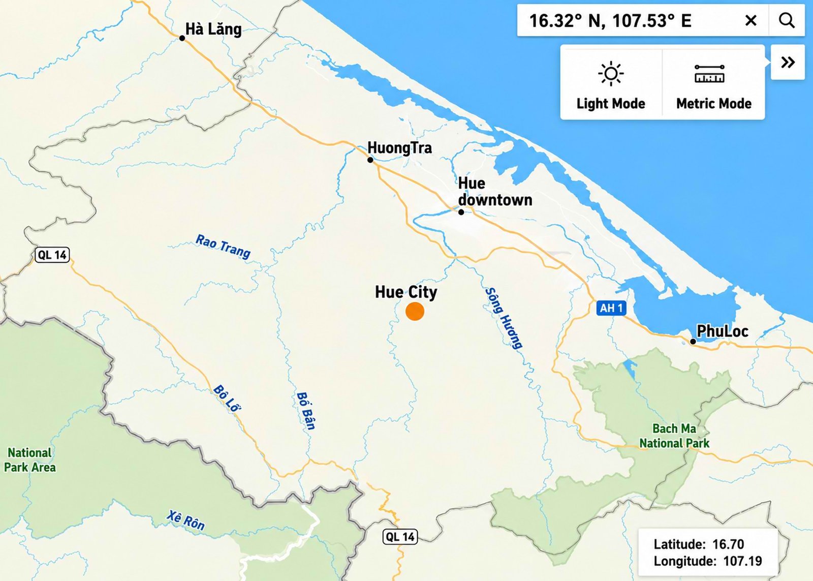
Fig. 1. Study area – Hue City, Vietnam.

Table 1

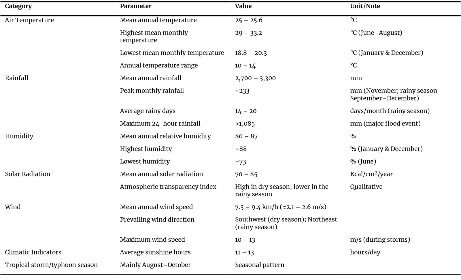
Table 1. The weather and climate profiles of Hue City.

These are the platforms that serve meteorological and solar data from satellites and climate models. The hourly dataset was extracted from January 1st, 2024, and May 30th, 2025, for a specific location (16.32° N, 107.53° E). Besides, Fig. 2 presents the 3D variations in optimal solar panel tilt angle in relation to SZA, ALLSKY_SFC_SW_DWN, and temporal variables, such as month, day, and hour. In the first plot, irradiance values range from 0 to over 1000 W/m², with the highest intensities occurring at SZA 25°, particularly between May and August, when the sun reaches its maximum altitude. The second plot displays daily patterns, where solar radiation peaks near 900–1000 W/m² at SZA 30° around 12:00 p.m., gradually decreasing to below 200 W/m² during early morning and late afternoon hours. The third plot shows hourly fluctuations across the day, confirming that irradiance reaches its maximum between 11:00 a.m. and 1:00 p.m., corresponding to minimal SZA values. Across all three plots, solar irradiance is inversely proportional to SZA, demonstrating a consistent dependency on solar geometry and time. Collectively, these visualizations underscore how diurnal and seasonal dynamics govern surface solar energy distribution.

Figure 2

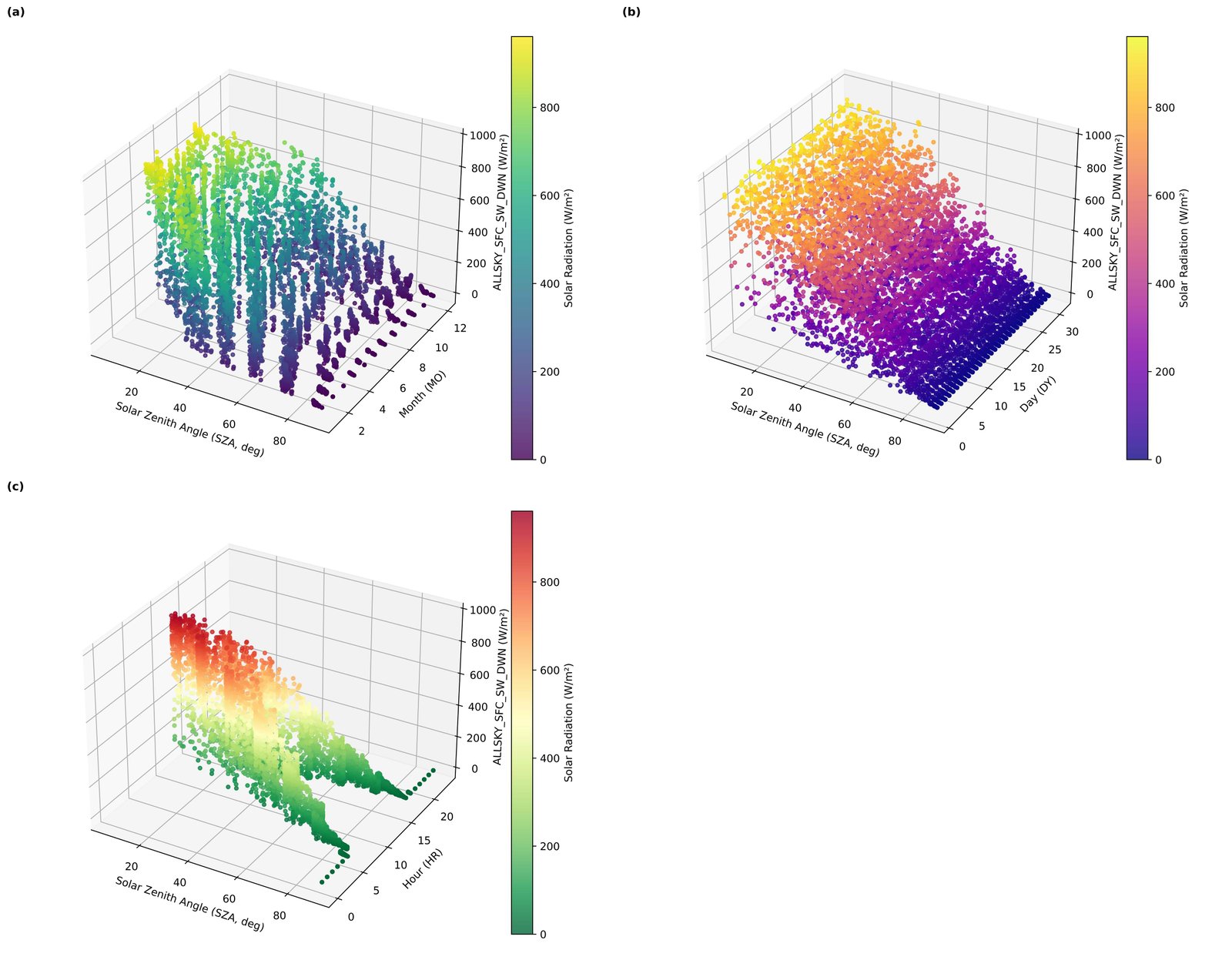
Fig. 2. Optimal tilt angle variations per (a) hour, (b) day, and (c) month for maximizing solar irradiance capture, surface solar energy distribution.

The dataset consists of seven input variables and one output variable used for modeling solar radiation under various atmospheric conditions. The study employs seven physically meaningful input variables widely used in solar radiation and atmospheric modeling, together with one output variable representing surface solar irradiance.

Input variables (predictors):

CLRSKY_SFC_SW_DWN: This parameter describes the theoretical solar radiation reaching the surface under cloud-free conditions. It supplies a physical baseline for predicted actual radiation and is commonly used in radiative transfer and solar energy models as a reference component.
ALLSKY_KT: The clearness index describes atmospheric transparency by relating actual surface radiation to extraterrestrial radiation. It captures the integrated effects of clouds, aerosols, and atmospheric attenuation, and is widely applied in empirical and machine learning–based solar prediction studies.
ALLSKY_SRF_ALB: Surface albedo quantifies the fraction of incoming solar radiation reflected by the ground. It influences the surface radiation balance and energy exchange processes, making it a key parameter in land–atmosphere interaction modeling.
WS10M: Wind speed affects atmospheric mixing, cloud movement, and heat transfer processes, indirectly influencing surface radiation variability.
T2M: Near-surface temperature is strongly linked to radiative fluxes and atmospheric stability, and is commonly included in solar radiation forecasting models.
QV2M: Water vapor is a major absorber of shortwave radiation. Specific humidity, therefore, directly influences atmospheric transmissivity and surface irradiance.
SZA: The solar zenith angle determines the sun’s geometric position relative to the Earth’s surface and directly controls the path length of solar radiation through the atmosphere. It is a fundamental astronomical parameter in radiation modeling.

Output variable:

ALLSKY_SFC_SW_DWN: This variable describes the total incoming shortwave radiation at the earth’s surface under real atmospheric conditions (including clouds). It is widely applied as a target variable in solar energy assessment, climate studies, and renewable energy forecasting.

The collected variables are physically grounded in radiative transfer theory and surface energy balance principles, ensuring both scientific justification and relevance for estimation of modeling applications.

The dataset comprises 6,421 hourly observations for seven input variables and one output parameter, ensuring sufficient temporal variability for robust modeling. To preserve the temporal structure of the time series and avoid data leakage, a strict chronological split was adopted rather than random sampling. Accordingly, the first 70% of the observations (4,495 hours) were used for model training, while the remaining 30% (1,926 hours) were reserved for independent testing, following established machine learning practices[31,32]. This proportion provides sufficient data for the model to learn the underlying relationships among the seven predictors while preserving an independent subset for unbiased evaluation of generalization performance. Such a split is appropriate for a dataset of this size, maintaining statistical reliability and validation stability.

Before model development, the seven input variables were normalized to improve numerical stability and computational efficiency.

Because the predictors differ in physical units and magnitudes, scaling them to a common range prevents dominance by larger-scale variables, facilitates gradient-based optimization, and enhances the overall predictive accuracy.

3.2. Baseline machine learning models

Three widely used machine learning models were implemented as baselines:

LS model: Used as a statistical baseline for capturing linear relationships between solar radiation and meteorological predictors. SVM model: Employed with a radial basis function (RBF) kernel to account for nonlinear interactions. SVM is known for its robustness in small- to medium-sized datasets.

XGB model: A gradient-boosted ensemble model optimized for handling high-dimensional and nonlinear features. Hyperparameters were fine-tuned for stability and accuracy: n_estimators = 70, learning_rate = 0.05, max_depth = 6, random_state = 42.

3.3. Deep learning models

To handle sequential dependencies and nonlinear dynamics in solar radiation time-series data, two neural network models were developed in Table 2.

Table 2

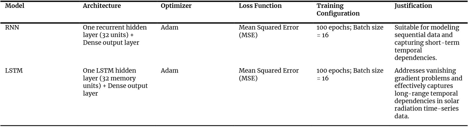
Table 2. Configuration and training parameters of RNN and LSTM models.

3.4. Hybrid model framework

To overcome the limitations of individual models, hybrid models were designed using a residual learning framework:

Step 1: Base Model Prediction A machine learning model (LS, SVM, or XGB) generates initial forecasts.

Step 2: Residual Error Modeling. Prediction errors (residuals = actual – predicted) are extracted from the training phase.

Step 3: Sequence Model Learning RNN or LSTM is trained on the residual errors to capture temporal structures in the prediction gaps.

Step 4: Hybrid Forecast. Final predictions are computed as the sum of the base model forecast and the sequence model residual forecast.

Six hybrid variants were implemented: XGB-RNN, XGB-LSTM, LS-RNN, LS-LSTM, SVM-RNN, SVM-LSTM. This two-stage hybrid design combines the strength of deterministic models with the temporal learning capabilities of RNN/LSTM.

All experiments were implemented in Python 3 with libraries including scikit-learn, TensorFlow/Keras, XGB, and NumPy. In addition, Table 3 optimizes configurations, architectures, and training settings of statistical, ML, DL, and hybrid forecasting models deployed.

Table 3

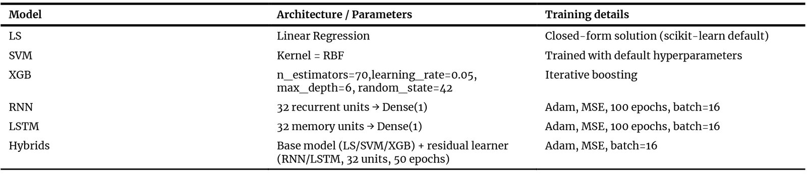
Table 3. Model configuration summary.

3.5. Model evaluation

The performance of all models was assessed using three metrics:

\[ RMSE\ =\sqrt{\frac{1}{n} \sum_{i=1}^{n} \left(y_i-\ {\ hat{y}}_i \right)} \]

\[ MAE=\frac{1}{n}\sum_{i=1}^{n}\left|y_i-\ {\hat{y}}_i\right| \]

\[ R^2=1-\frac{\sum_{i=1}^{n}\left(y_i-\ {\ hat{y}}_i\right)^2}{\sum_{i=1}^{n}\left(y_i-\ \bar{y}\right)^2} \]

\[ CC\ =\ 1-\frac{\sum_{t=1}^{n}{(y_i-\bar{y_i})}({\hat{y}}_i-\bar{{\hat{y}}_i})}{\sum_{t=1}^{n}\left(y_i-\bar{y_i}\right)^2\ ast\ \sum_{t=1}^{n}\left({\hat{y}}_i-\bar{{\hat{y}}_i}\right)^2} \]

where \(y_i\), \({\hat{y}}_i\),(\(\bar{y_i}\)), (\(\bar{\ {\hat{y}}_i}\)), n describe the observed values, the predicted values, the mean of the observed values, the mean of the predicted values, and the total number of observations, respectively.

The study workflow is illustrated in Fig. 3. The process starts with data acquisition and preprocessing, followed by exploratory data analysis and the design of an incremental training strategy. ML, DL, and hybrid models are deployed and critiqued using defined performance indicators. Simulation and statistical analysis are conducted, with calibration performed iteratively until satisfactory results are achieved.

Figure 3

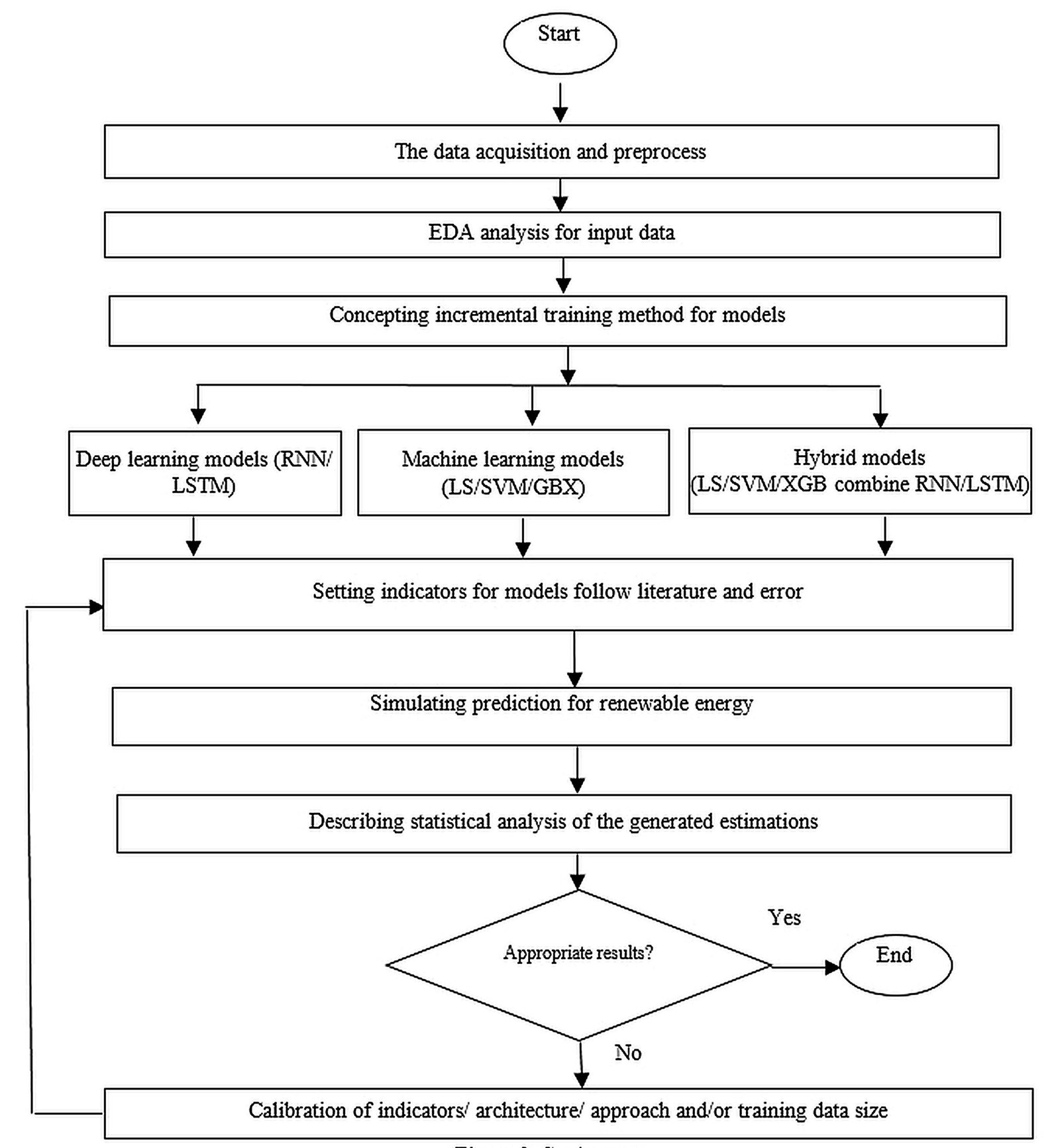
Fig. 3. Study steps.

4. Results and discussions

This paper explores the prediction capability of ML, DL, and hybrid models for solar radiation and meteorological variables. Using a dataset of 6,421 hourly observations across eight features, traditional, deep learning, and hybrid approaches are systematically compared.

As shown in Table 4 presents the mean, std, min, and max values of all variables. CLRSKY_SFC_SW_DWN shows a mean of 507.31 W/m², ranging from 2.40 to 982.00 W/m², with a std of 309.16. ALLSKY_KT averages 0.38 (min 0.01, max 0.76; std 0.18), while ALLSKY_SRF_ALB has a mean of 0.07 with low variability (std 0.01). WS10M records a mean of 3.67 m/s (0.04–11.48; std 1.79). T2M averages 26.55 (15.43–38.67; std 4.08). QV2M has a mean of 17.39 (9.09–23.47; std 2.91). SZA averages 51.86° (5.75–89.43; std 23.21). ALLSKY_SFC_SW_DWN shows a mean of 335.05 W/m² (0.20–960.90; std 262.55).

Table 4

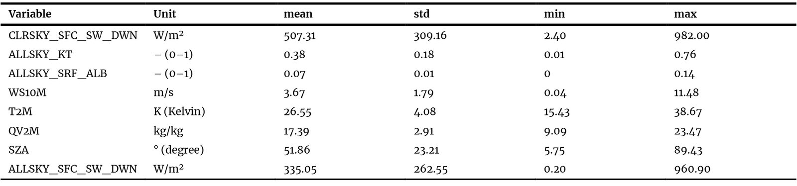
Table 4. Descriptive statistic.

In addition, Fig. 4 shows that KDE plots were used to evaluate distributional characteristics further. Both results show wide distributions for CLRSKY_SFC_SW_DWN and ALLSKY_SFC_SW_DWN, highlighting significant variability in solar radiation across clear and all-sky conditions. In comparison, ALLSKY_KT shows a bimodal distribution, corresponding to a cloud-to-clear-sky transition. Meanwhile, T2M and QV2M demonstrate relatively compact distributions, whereas WS10M displays skewness toward lower values. As expected, SZA spans a wide range, capturing daily and seasonal cycles. Supporting boxplots reinforce these trends, underscoring a more pronounced spread among radiation variables in comparison to the more consistent meteorological features, further highlighting the heterogeneous nature of solar-related data sets.

Figure 4

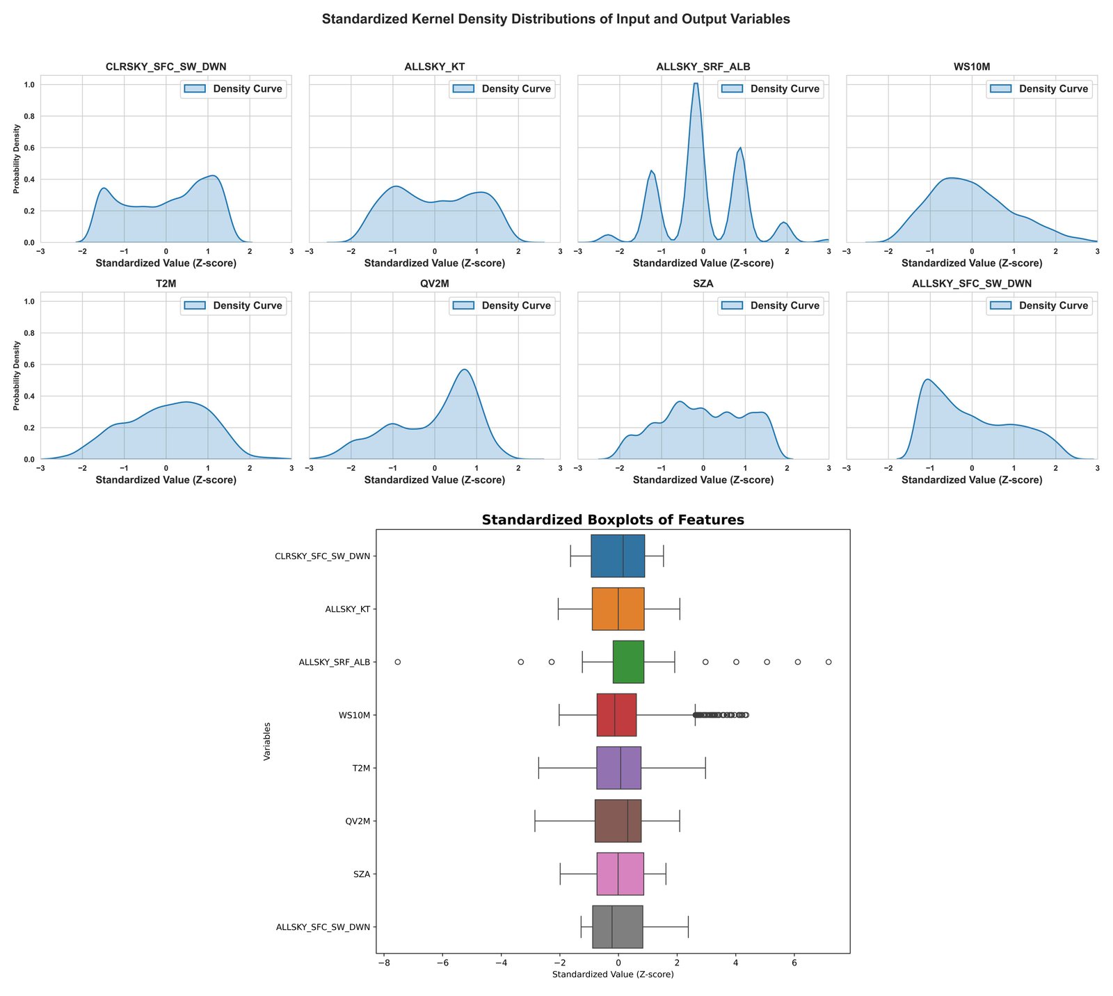
Fig. 4. KDE plots and boxplots of solar radiation and meteorological features.

Moving forward, Fig. 5 indicates that correlation analysis further elucidates interdependencies among features. Most impressively, CLRSKY_SFC_SW_DWN almost perfectly correlates with ALLSKY_SFC_SW_DWN (r = 0.97), confirming that clear-sky and all-sky radiation have the same pattern. Similarly, ALLSKY_KT exhibits strong positive correlations with both CLRSKY_SFC_SW_DWN (r = 0.70) and ALLSKY_SFC_SW_DWN (r = 0.67), consistent with its role as a clearness index. Conversely, SZA shows strong negative correlations with radiation variables (r = −0.73 and −0.84, respectively), in agreement with solar geometry principles. Among meteorological parameters, T2M and QV2M display a strong positive correlation (r = 0.87), whereas WS10M remains weakly related (<0.20), highlighting its independent variability.

Figure 5

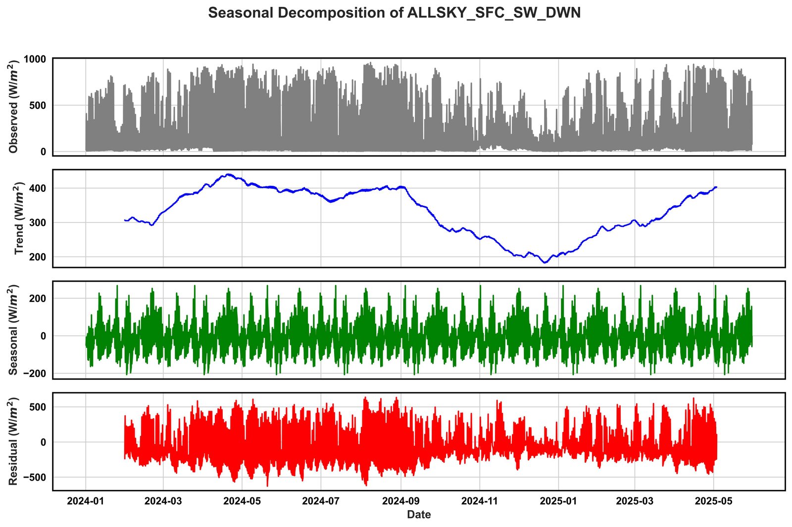
Fig. 5. Seasonal decomposition of ALLSKY_SFC_SW_DWN.

Similarly, Fig. 6 displays the seasonal decomposition of ALLSKY_SFC_SW_DWN, which further illustrates these dynamics. The trend component reveals a distinct annual cycle, increasing in early 2024, peaking mid-year at approximately 450 W/m², and subsequently declining toward late 2024 before recovering in 2025. The seasonal component captures periodic oscillations associated with solar cycles, while residuals reflect short-term fluctuations of up to ±500 W/m².

Figure 6

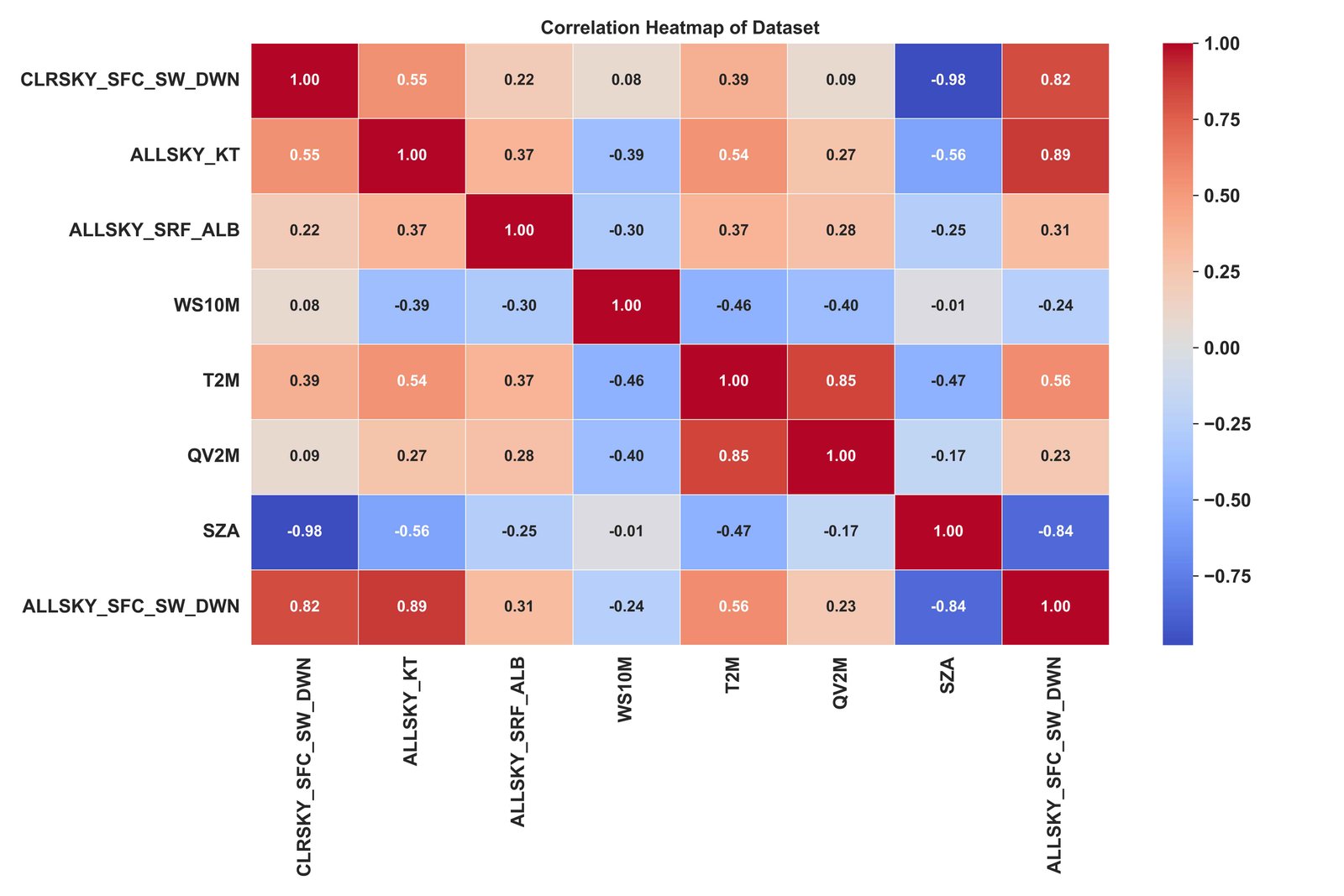
Fig. 6. Correlation matrix of solar radiation and meteorological features.

Collectively, these results highlight the combined influence of solar geometry and atmospheric variability.

As presented in Table 5 and Fig. 7, clear performance differences are observed among the standalone and hybrid models, highlighting the influence of algorithmic structure on solar radiation prediction. Among the individual models, XGB delivers the strongest performance (RMSE = 11.31, MAE = 8.89, R² = 0.99), substantially outperforming SVM (RMSE = 52.07, R² = 0.96) and LSTM (RMSE = 66.40, R² = 0.93). RNN achieves the superior performance of XGB is consistent with prior studies cited in the Literature Review, which report that gradient-boosting frameworks effectively capture nonlinear relationships and complex feature interactions in solar radiation modeling. Unlike SVM, which is sensitive to kernel configuration and parameter tuning, XGB iteratively minimizes residual errors through ensemble learning, improving robustness and reducing bias. The comparatively weaker standalone LSTM and RNN results suggest that, in this dataset, nonlinear feature interactions among physically grounded predictors (e.g., clearness index, solar zenith angle, humidity) are more dominant than long-range temporal dependencies. This partially contrasts with studies emphasizing deep recurrent networks as superior for time-series forecasting; however, those works often rely on longer temporal sequences or purely sequential inputs. Herein, the predictors already encode strong physical information, which may reduce the marginal benefit of standalone deep architectures.

Figure 7

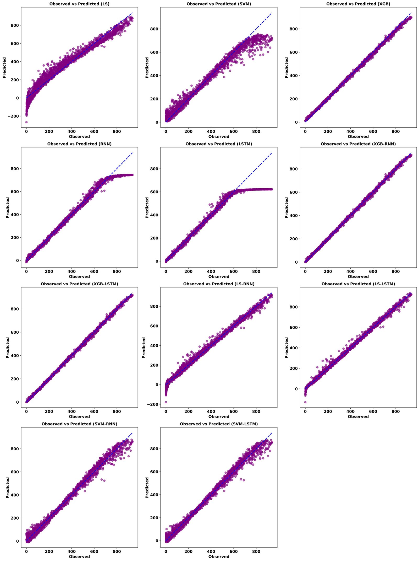
Fig. 7. Scatter plots of testing phase for the models.

Table 5

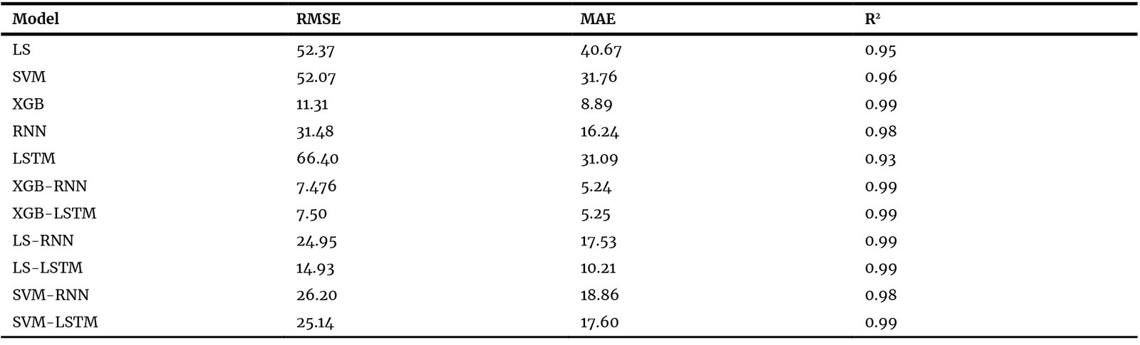
Table 5. Accuracy matrix of model parameters.

Hybrid models produce further improvements. XGB-RNN (RMSE = 7.48, R² = 0.99) and XGB-LSTM (RMSE = 7.51, R² = 0.99) gain the highest accuracy, revealing that residual learning increases predictive precision. This aligns with recent hybrid modeling literature suggesting that combining deterministic ensemble learners with sequence-based networks be able to capture both structural nonlinearities and temporal residual patterns. LS-LSTM and SVM-LSTM also outperform their standalone counterparts, supporting the general effectiveness of hybridization, though they remain less competitive than XGB-based hybrids.

The scatter plots reinforce these findings: XGB hybrids cluster most tightly along the 1:1 line, indicating minimal dispersion and systematic bias, whereas SVM and standalone LSTM exhibit greater spread. Overall, the results support the literature advocating ensemble-based and hybrid frameworks for solar radiation forecasting, while also suggesting that, for physically informed predictor sets, boosting-based methods may be more influential than deep recurrent networks alone.

In addition, Fig. 8 shows feature-level analysis of XGB-LSTM performance, which reveals high predictive accuracy for deterministic parameters such as SZA (R² = 0.99), CLRSKY_SFC_SW_DWN (R² = 0.99), and ALLSKY_KT (R² = 0.993). Likewise, T2M (R² = 0.95) and QV2M (R² = 0.95) are reliably predicted. In contrast, ALLSKY_SRF_ALB (R² = 0.71) and WS10M (R² = 0.67) exhibit weaker predictive accuracy, reflecting the stochastic and localized nature of albedo and wind processes. These findings underscore the challenges of modeling highly variable parameters.

Figure 8

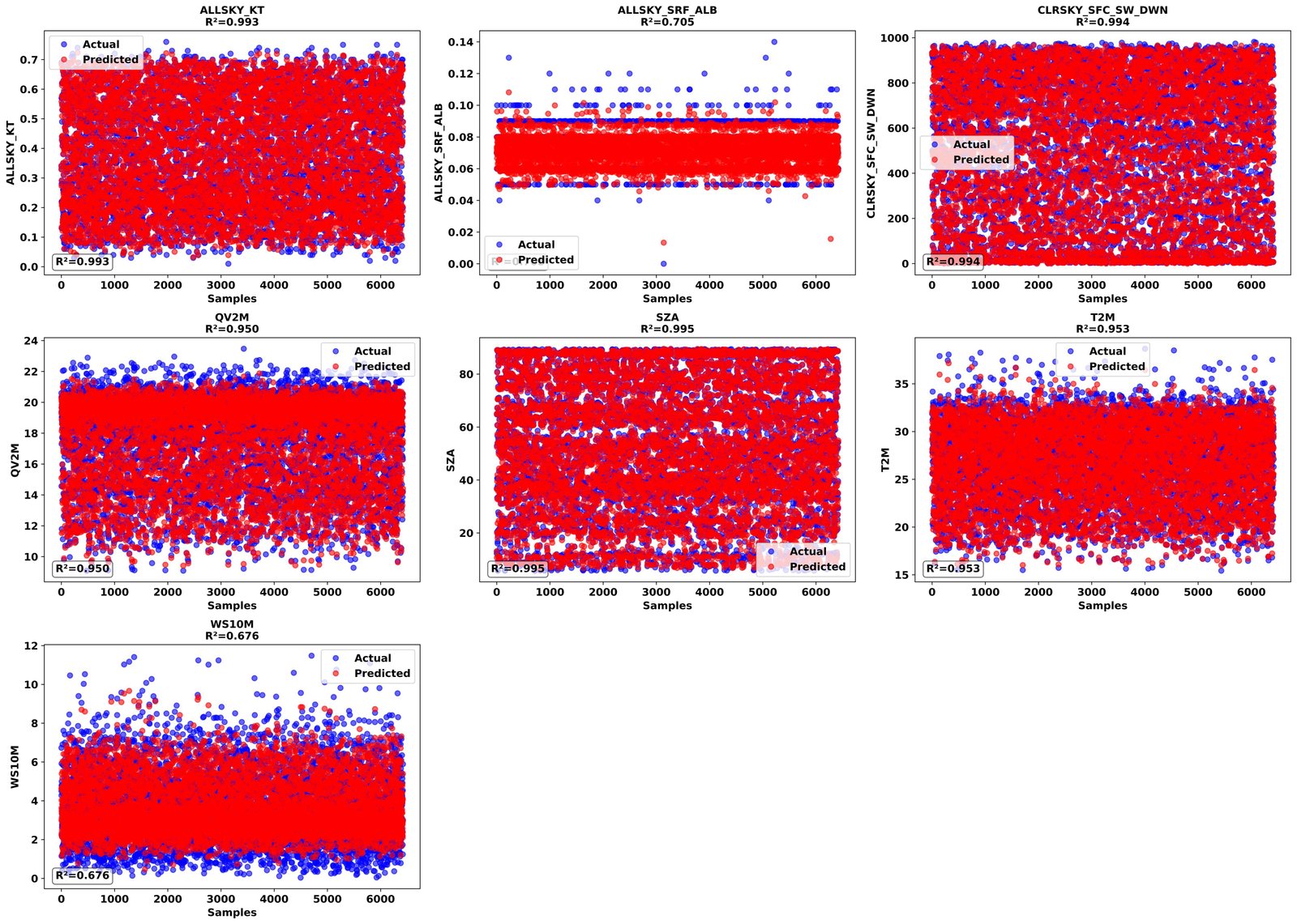
Fig. 8. Actual versus predicted values for individual features using the XGB-LSTM model.

Furthermore, Fig. 9 shows the Taylor diagram consolidates performance comparisons across 12 models (LS, SVM, XGB, RNN, LSTM, XGB-RNN, XGB-LSTM, LS-RNN, LS-LSTM, SVM-RNN, SVM-LSTM, and Observation). Most models cluster near the observation reference, with standard deviations between 200 and 250 and correlations with CC values approaching 1. Notably, hybrid approaches such as XGB-LSTM and SVM-LSTM align most closely with observed values, thereby validating their predictive robustness.

Figure 9

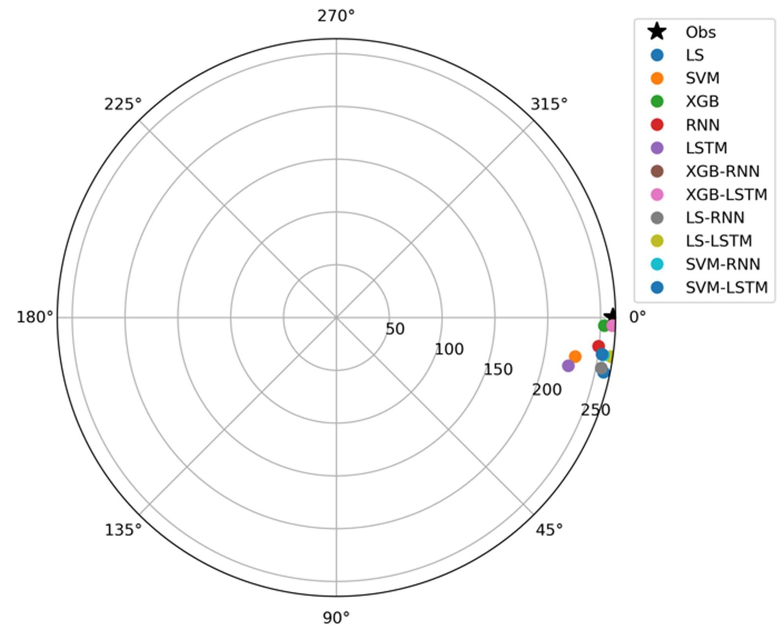
Fig. 9. Taylor diagram comparing the performance of standalone and hybrid models against observations.

Figure 10 displays the LIME-based local explanation chart, which illustrates the relative contributions of meteorological and solar geometry features to the XGB-LSTM prediction. The dominant positive contribution of ALLSKY_KT ( 0.71) reflects the clearness index’s direct representation of atmospheric transmissivity. Physically, higher KT values indicate reduced cloud cover and aerosol scattering, allowing greater shortwave radiation to reach the surface. Its leading influence is therefore consistent with radiative transfer theory and confirms that the hybrid model prioritizes atmospheric clarity as the primary driver of surface irradiance.

Figure 10

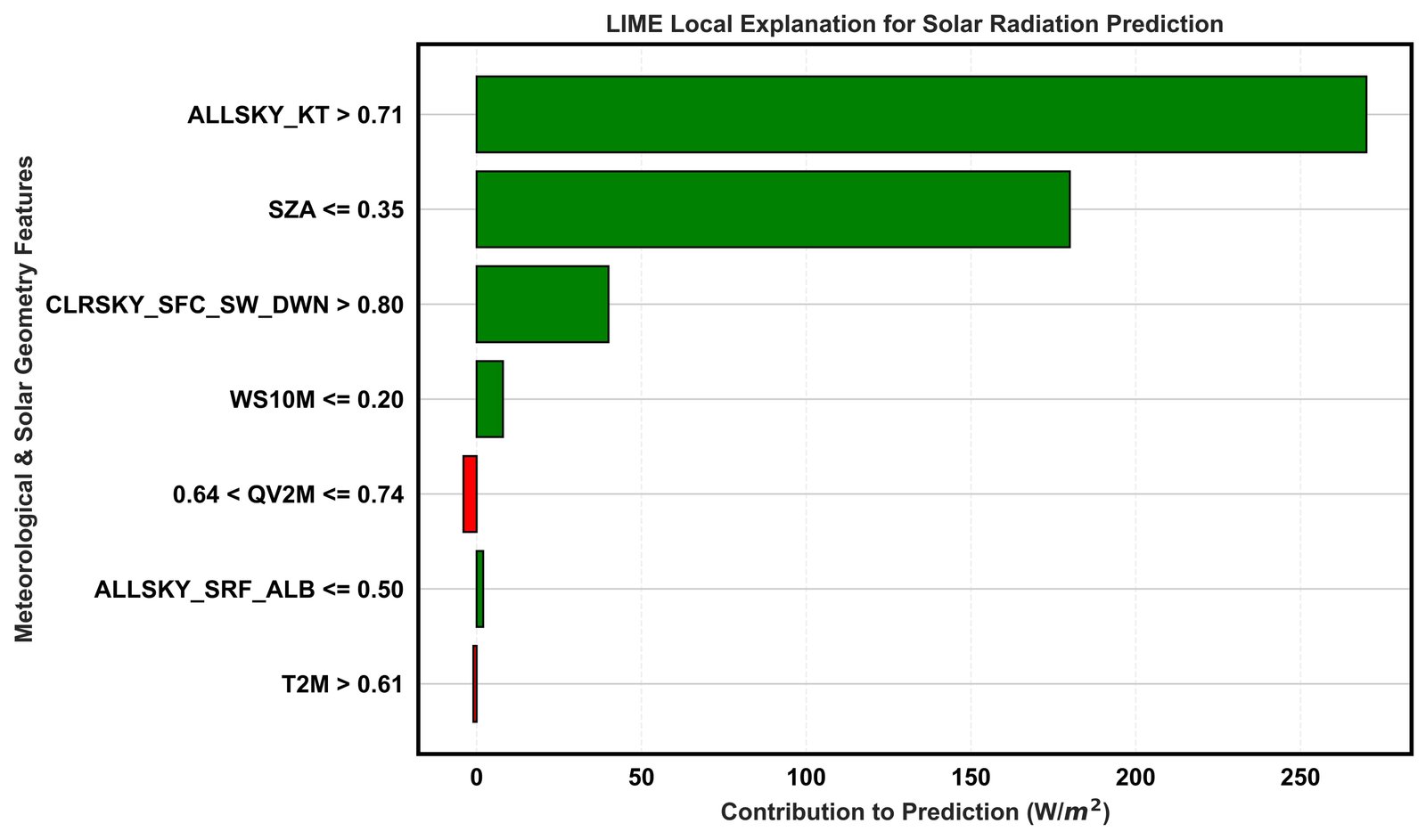
Fig. 10. LIME based feature importance for the XGB-LSTM model.

Similarly, the strong contribution of low SZA ( 0.35) aligns with solar geometry fundamentals. A smaller solar zenith angle corresponds to a shorter optical air mass path, reducing scattering and absorption losses, which increases incoming radiation. This confirms that the model appropriately encodes astronomical controls on irradiance variability.

The moderate role of CLRSKY_SFC_SW_DWN indicates that clear-sky radiation provides a physically constrained upper bound for potential solar input, supporting operational forecasting benchmarks. In contrast, variables such as WS10M, QV2M, and T2M exhibit smaller contributions because they influence radiation indirectly, through cloud formation, moisture content, or boundary-layer dynamics, rather than directly determining radiative flux.

From an operational standpoint, this hierarchy of importance requires that real-time forecasting systems prioritize accurate cloud and aerosol monitoring, as improvements in atmospheric transparency measurements would yield the greatest predictive gains.

Finally, Fig. 11 displays a set of seven 3D scatter plots that further confirms the temporal learning capacity of XGB-LSTM. With axes defined as time (HR), actual values, and estimated values, these plots demonstrate strong. diagonal clustering across all predictor variables: (1) ALLSKY_KT, (2) ALLSKY_SRF_AER, (3) CLRSKY_SFC_SW_DWN, (4) O2VM, (5) SZA, (6) T2M, and (7) WS10M. These results indicate that the hybrid model effectively captures diurnal patterns between 06:00 and 18:00, thereby reinforcing its robustness in mapping predictor–response relationships.

Figure 11

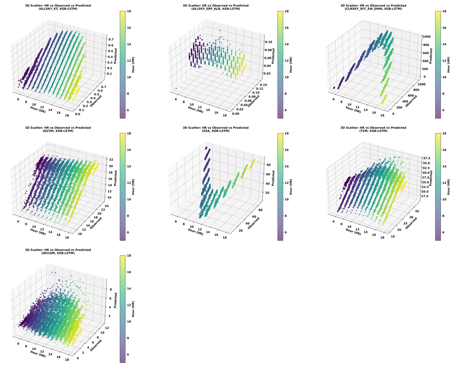
Fig. 11. 3D scatter plots of observed versus predicted values for predictor variables using the XGB-LSTM model.

The superior performance of XGB-RNN and XGB-LSTM can be explained by the complementary strengths of their components rather than by algorithmic complexity alone. XGB is highly effective at capturing nonlinear interactions among physically meaningful predictors such as clearness index, solar zenith angle, humidity, temperature, and wind speed. As discussed in the Literature Review, gradient-boosting models iteratively minimize residual errors and handle multicollinearity robustly, making them particularly suitable for solar radiation modeling where atmospheric processes are nonlinear and interdependent.

However, while XGB captures the dominant structural relationships, short-term temporal fluctuations may remain in the residuals. The RNN and LSTM networks are then trained to model these residual sequences, learning temporal dependencies that standalone boosting models cannot fully represent. This residual-learning mechanism reduces noise and mitigates overfitting, explaining why hybrid models outperform standalone LSTM and SVM approaches. The findings, therefore, align with previous studies advocating hybrid ensemble–recurrent frameworks for enhancing forecasting accuracy. Unlike conventional hybrid models that directly stack predictors, this study adopts a structured residual-learning framework in which deterministic models first capture nonlinear relationships and recurrent networks model only the remaining temporal errors. This decomposition reduces noise propagation, enhances stability, and systematically compares six hybrid variants under a unified evaluation matrix.

Feature-level analysis, moreover, underscores these findings. Deterministic parameters controlled by physical laws, including SZA, CLRSKY_SFC_SW_DWN, and ALLSKY_KT, were predicted very accurately, highlighting the model’s ability to capture systematic patterns. On the other hand, more stochastic variables like ALLSKY_SRF_ALB and WS10M had weaker correlations, underscoring the challenges of modeling localized and highly variable processes. As a result, future work could also integrate other explanatory features, such as land cover, pressure gradients, or spatially distributed datasets, to enhance predictive skill. Both the Taylor diagram and 3D scatter plots confirm model robustness, showing excellent correspondence between observed and predicted values during the daytime. Overall, these results strongly motivate embracing XGB-based hybrids as a default basis for solar forecasting, climate applications, and atmospheric research, yielding essential advantages over traditional single-model approaches.

Finally, the findings of this study have strong implications for setting up PV systems in Hue City, a region characterized by tropical monsoon conditions with significant cloud cover and seasonal variability. Using 6,421 hourly observations and an advanced hybrid XGB-LSTM model, the study provides accurate predictions of solar radiation with R² values exceeding 0.999. The average all-sky solar radiation (335.05 W/m²) confirms Hue’s strong potential for PV deployment despite variable weather.

The analysis of solar zenith angle, clearness index, and optimal tilt angle, ranging from 25° to 30° annually, offers valuable guidance for PV orientation and design. Additionally, the hybrid models’ accuracy allows for real-time solar forecasting, which is imperative for grid management and energy planning. These insights support policymakers and investors in optimizing PV siting, tilt configuration, and seasonal energy output, contributing to sustainable energy transition and climate resilience in central Vietnam.

5. Conclusion

The study presented ML, DL, and their hybrid approaches for anticipating solar radiation and associated meteorological factors from 6,421 hourly observations. These outcomes underscore the supremacy of hybrid models with XGB-RNN and XGB-LSTM, producing R² above 0.99 with minimal RMSE and MAE. These results confirm the value of merging gradient boosting’s nonlinear processing with recurrent networks’ time-wise learning. Deterministic features such as SZA, ALLSKY_KT, and CLRSKY_SFC_SW_DWN were modeled well, whereas highly stochastic parameters such as WS10M and ALLSKY_SRF_ALB were more challenging. Moreover, the key research has strong implications for setting up PV systems in Hue City, which has strong potential for efficient PV deployment and energy planning.

Although the dataset covers one region and period, the methodology is inherently transferable. It relies on physically based predictors relevant across climates and deploys a modular hybrid framework (XGB + RNN/LSTM) that can be retrained with local data. Multi-regional and federated schemes further enhance scalability and cross-climate applicability.

Hybrid models require higher computational resources, potentially limiting real-time implementation. While LIME enhances transparency, full interpretability remains challenging due to the semi-black-box nature of hybrid architectures. Additionally, excluding variables such as aerosol concentration or land cover may have constrained predictive performance.

Future research should extend to a wider range of geographic regions and climatic regimes to rigorously evaluate the robustness and external validity of the proposed simulation framework. Incorporating additional predictors, such as satellite-derived aerosol concentrations or atmospheric pressure gradients, may further enhance model conduction, particularly under conditions characterized by high radiation variability. From a methodological perspective, attention-based mechanisms or transformer architectures could be explored to more effectively capture temporal relationships in models compared with conventional recurrent networks.

Funding

This research received no external funding.

Acknowledgement

The authors would like to express their sincere gratitude to Damien Crapon and Alexandre Vaux, students from École Centrale Lyon, Lyon, France, for their valuable assistance in identifying and collecting the database used in this research.

Author Contributions

HongGiang Nguyen, VietNguyenHoang Tran: Writing – original draft, Visualization, Resources, Methodology, Investigation, Software, Resources, Data curation. Vinh V. Le, XuanCuong Ngo: Writing – review & editing, Writing – original draft, Supervision, Resources, Methodology, Conceptualization.

Declaration of competing interest

The authors declare no conflicts of interest.

References

Qudrat-Ullah, H., Myth: Renewable Energy is Too Intermittent to Be Reliable?, in Sustainable Energy: A Myth or Reality. 2024, Springer. p. 17-47. https://doi.org/10.1007/978-3-031-59733-6_2
Singh, S. and S. Singh, Advancements and challenges in integrating renewable energy sources into distribution grid systems: A comprehensive review. Journal of Energy Resources Technology, 2024. 146(9): p. 090801. https://doi.org/10.1115/1.4065503
Howlader, A.S., Machine learning applications in renewable energy: predictive analytics for solar cell performance optimization and energy yield forecasting. american journal of scholarly research and innovation, 2025. 4(01): p. 392-427. https://doi.org/10.63125/asxzy065
Jannah, N., et al., Recent Advances and Future Challenges of Solar Power Generation Forecasting. IEEE Access, 2024. https://doi.org/10.1109/ACCESS.2024.3496120
Yang, D. and J. Kleissl, Solar irradiance and photovoltaic power forecasting. 2024: CRC Press. https://doi.org/10.1201/9781003203971
Verma, S., Y.L. Kameswari, and S. Kumar, A review on environmental parameters monitoring systems for power generation estimation from renewable energy systems. BioNanoScience, 2024. 14(4): p. 3864-3888. https://doi.org/10.1007/s12668-024-01358-4
Piekarski, M., Motivation, counterfactual predictions and constraints: normativity of predictive mechanisms. Synthese, 2022. 200(5): p. 352. https://doi.org/10.1007/s11229-022-03837-1
Balla, J. and M.S. Hagger, Protection motivation theory and health behaviour: conceptual review, discussion of limitations, and recommendations for best practice and future research. Health Psychology Review, 2025. 19(1): p. 145-171. https://doi.org/10.1080/17437199.2024.2413011
Ahmed, S.F., et al., Deep learning modelling techniques: current progress, applications, advantages, and challenges. Artificial Intelligence Review, 2023. 56(11): p. 13521-13617. https://doi.org/10.1007/s10462-023-10466-8
Zhou, W., Z. Yan, and L. Zhang, A comparative study of 11 non-linear regression models highlighting autoencoder, DBN, and SVR, enhanced by SHAP importance analysis in soybean branching prediction. Scientific Reports, 2024. 14(1): p. 5905. https://doi.org/10.1038/s41598-024-55243-x
Soromotin, A.V., D.A. Martyushev, and J.L.J. Pereira, On the application of machine learning algorithms in predicting the permeability of oil reservoirs. Artificial Intelligence in Geosciences, 2025: p. 100126. https://doi.org/10.1016/j.aiig.2025.100126
Kocher, G. and G. Kumar, Machine learning and deep learning methods for intrusion detection systems: recent developments and challenges. Soft Computing, 2021. 25(15): p. 9731-9763. https://doi.org/10.1007/s00500-021-05893-0
Al-Nouti, A.F., M. Fu, and N.D. Bokde, Reservoir operation based machine learning models: comprehensive review for limitations, research gap, and possible future research direction. Knowledge-Based Engineering and Sciences, 2024. 5(2): p. 75-139. https://doi.org/10.51526/kbes.2024.5.2.75-139
Zhang, J., et al., Interpretable machine learning models for evaluating strength of ternary geopolymers. Artificial Intelligence in Geosciences, 2025: p. 100128. https://doi.org/10.1016/j.aiig.2025.100128
Khan, S., et al., Comparative analysis of deep neural network architectures for renewable energy forecasting: enhancing accuracy with meteorological and time-based features. Discover Sustainability, 2024. 5(1): p. 533. https://doi.org/10.1007/s43621-024-00783-5
Chen, S., et al., Foundation models for weather and climate data understanding: A comprehensive survey. arXiv preprint arXiv:2312.03014, 2023. https://doi.org/10.48550/arXiv.2312.03014
Martinsen, I., et al., Quantifying uncertainty in foraminifera classification: How deep learning methods compare to human experts. Artificial Intelligence in Geosciences, 2025: p. 100145. https://doi.org/10.1016/j.aiig.2025.100145
Javed, H., F. Eid, S. El-Sappagh, and T. Abuhmed, Sustainable energy management in the AI era: a comprehensive analysis of ML and DL approaches. Computing, 2025. 107(6): p. 132. https://doi.org/10.1007/s00607-025-01485-0
Asif, S., et al., Advancements and prospects of machine learning in medical diagnostics: unveiling the future of diagnostic precision. Archives of Computational Methods in Engineering, 2025. 32(2): p. 853-883. https://doi.org/10.1007/s11831-024-10148-w
Nsulangi, P.T., W.E. Ngongi, J.M. Kafuku, and G.Z. Liang, Comparison of Processing Speed of NRS-ANN Hybrid and ANN Models for Oil Production Rate Estimation of Reservoir under Waterflooding. Artificial Intelligence in Geosciences, 2025: p. 100139. https://doi.org/10.1016/j.aiig.2025.100139
Le, V.V., H. Nguyen, and N.H. Ngu, Deep Learning Approaches for Estimating Maximum Wall Deflection in Excavations with Inconsistent Clay Stratigraphy. Artificial Intelligence in Geosciences, 2025: p. 100140. https://doi.org/10.1016/j.aiig.2025.100140
Li, X., et al., Probabilistic solar irradiance forecasting based on XGBoost. Energy Reports, 2022. 8: p. 1087-1095. https://doi.org/10.1016/j.egyr.2022.02.251
Bamisile, O., et al., Comprehensive assessment, review, and comparison of AI models for solar irradiance prediction based on different time/estimation intervals. Scientific Reports, 2022. 12(1): p. 9644. https://doi.org/10.1038/s41598-022-13652-w
Abisoye, B.O., Y. Sun, and Z. Wang, Machine learning forecasting model for solar energy radiation. International Journal of Computer Theory and Engineering, 2024. 16(2): p. 66-75. https://doi.org/10.7763/IJCTE.2024.V16.1355
Wang, Y., Y. Li, Y. Zheng, and W. Gao, Solar Radiation Forecasting with Hybrid Deep Learning Framework Integrating Feature Factorization. HUMAN-CENTRIC COMPUTING AND INFORMATION SCIENCES, 2025. 15. https://doi.org/10.22967/HCIS.2025.15.009
Xu, Y., X. Ji, and Z. Zhu, A photovoltaic power forecasting method based on the LSTM-XGBoost-EEDA-SO model. Scientific Reports, 2025. 15(1): p. 30177. https://doi.org/10.1038/s41598-025-16368-9
Didavi, K.B.A., R.G. Agbokpanzo, and B.M. Agbomahena, LSTM and XGBoost models for 24-hour ahead forecast of PV power from direct irradiation. Renewable Energy Research and Applications, 2024. 5(2): p. 229-241. https://doi.org/10.22044/rera.2023.12880.1209
Moradzadeh, A., et al., Generalized global solar radiation forecasting model via cyber-secure deep federated learning. Environmental Science and Pollution Research, 2024. 31(12): p. 18281-18295. https://doi.org/10.1007/s11356-023-30224-1
https://power.larc.nasa.gov/data-access-viewer/. [cited 2025 Agust 01st].
https://nchmf.gov.vn/kttvsiteE/en-US/2/index.html. [cited 2025 August 5th].
Vrigazova, B., The proportion for splitting data into training and test set for the bootstrap in classification problems. Business Systems Research: International Journal of the Society for Advancing Innovation and Research in Economy, 2021. 12(1): p. 228-242. https://doi.org/10.2478/bsrj-2021-0015
Singh, V., et al., Impact of train/test sample regimen on performance estimate stability of machine learning in cardiovascular imaging. Scientific reports, 2021. 11(1): p. 14490. https://doi.org/10.1038/s41598-021-93651-5

Get PDF (7.30 MB)

11
Total views

Citations

SHARE ON