Article | 10 June 2026
Volume 13 Issue 1 pp. 315-332 • doi: 10.15627/jd.2026.18
Optimizing Horizontal Shading Devices for Daylight Performance and Energy Efficiency in Kathmandu's Office Buildings: A Multi-Objective Study Under Current and Future Climate Scenarios
Prashant Chhetri*
Author affiliations
Department of Architecture, Institute of Engineering, Pulchowk Campus, Tribhuvan University, Lalitpur, 44700, Nepal
*Corresponding author.
prashantxytre@gmail.com (P. Chhetri)
History: Received 3 March 2026 | Revised 25 April 2026 | Accepted 3 May 2026 | Published online 10 June 2026
2383-8701/© 2026 The Author(s). Published by solarlits.com. This is an open access article distributed under the terms and conditions of the Creative Commons Attribution 4.0 License.
Citation: Prashant Chhetri, Optimizing Horizontal Shading Devices for Daylight Performance and Energy Efficiency in Kathmandu's Office Buildings: A Multi-Objective Study Under Current and Future Climate Scenarios, Journal of Daylighting, 13:1 (2026) 315-332. doi: 10.15627/jd.2026.18
Figures and tables
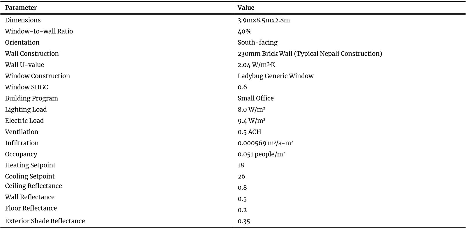 Table 1
 Table 2
 Table 3
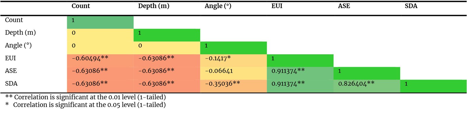 Table 4
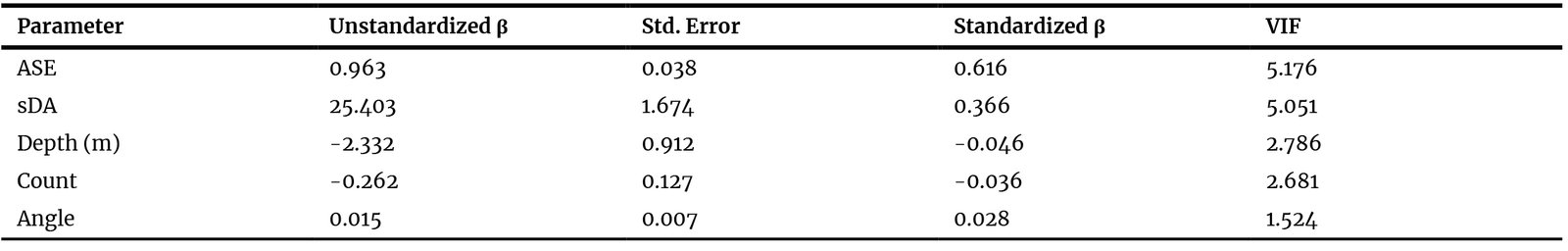 Table 5
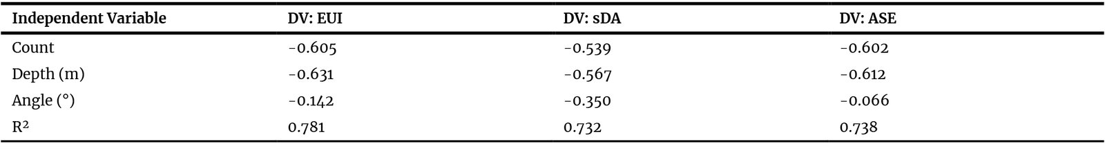 Table 6
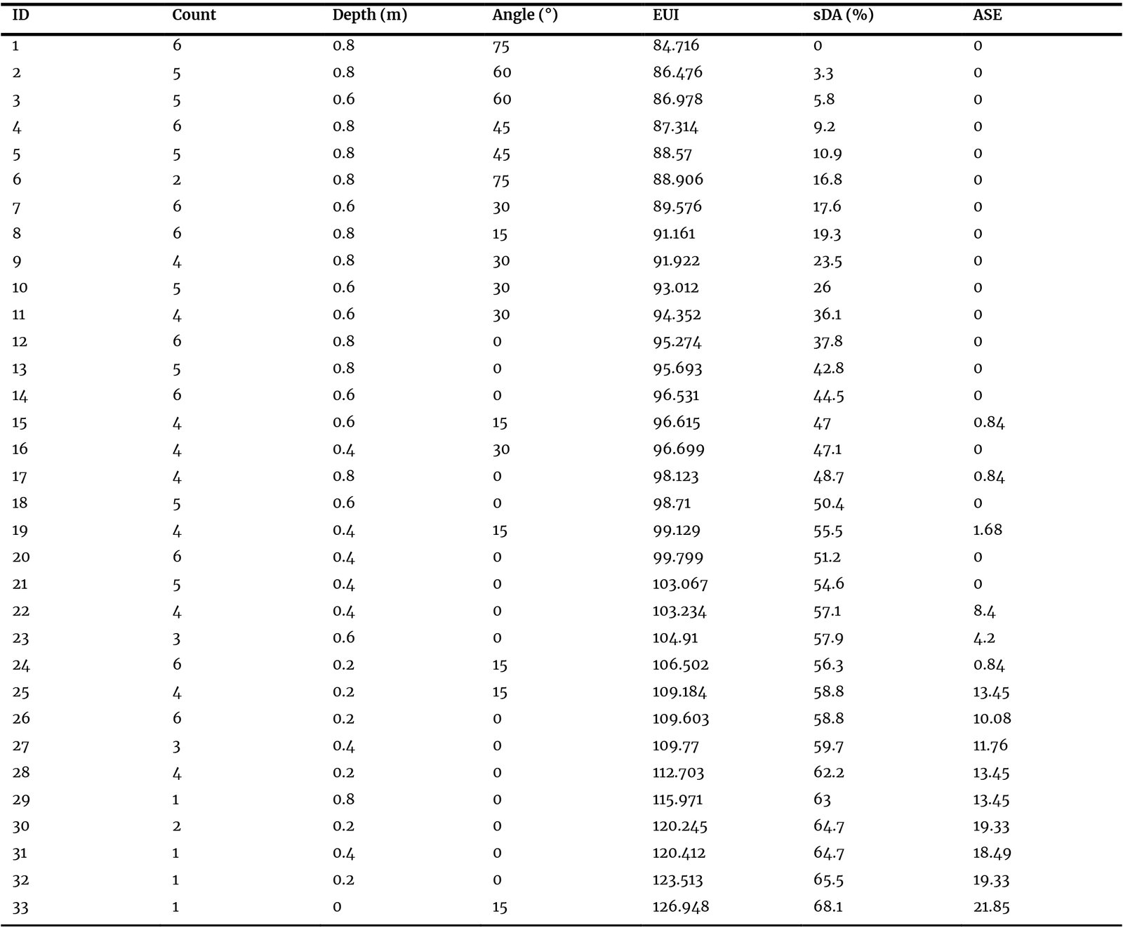 Table 7
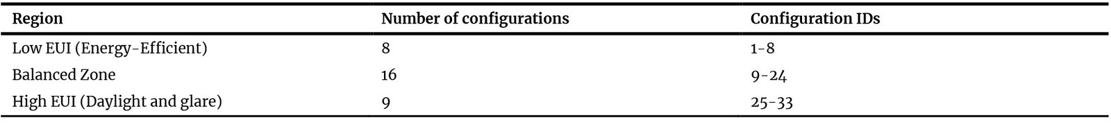 Table 8
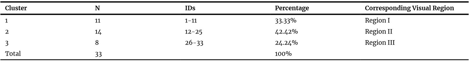 Table 9
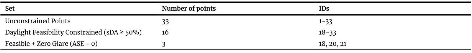 Table 10
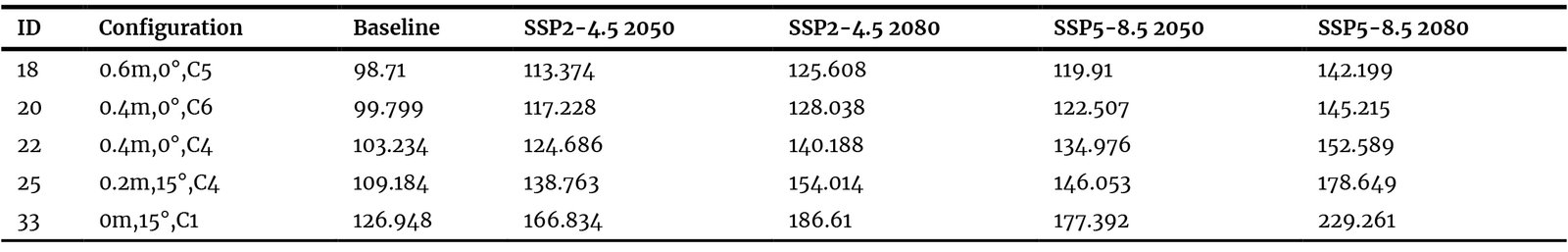 Table 11
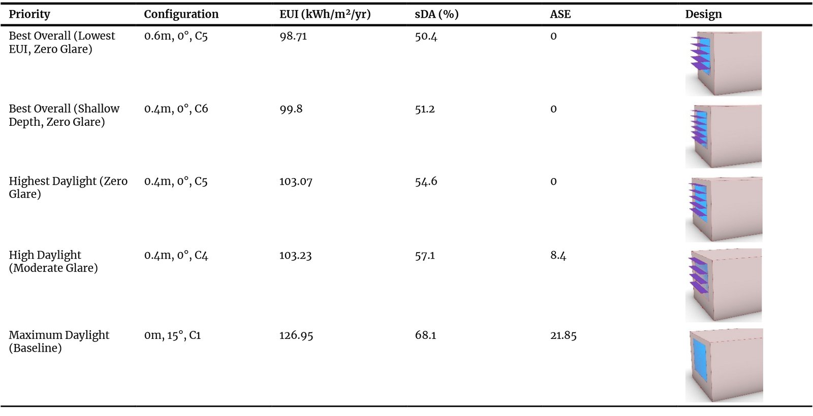 Table 12
Abstract
This study optimizes horizontal shading devices for south-facing office façades in Kathmandu to balance daylight, energy, and visual comfort under current and future climates. From 210 simulations varying shading count, depth, and angle, pairwise dominance checking identified 33 mathematically Pareto-optimal configurations. However, mathematical optimality does not guarantee practical suitability. When constrained by minimum daylight requirements (sDA ≥ 50%), the viable design space collapses to 16 feasible configurations, of which only 3 achieve zero glare (ASE = 0). K-means clustering validated three design strategies: Energy-Efficient (n=11) with low EUI and zero glare but limited daylight; Balanced (n=14) with good daylight, low glare, and moderate EUI; and Daylight-Optimal (n=8) with high daylight but high EUI and glare. The recommended configuration (0.4 m depth, 0° angle, 6 louvers) achieves 51.2% sDA with zero glare and 21% energy savings. Under future scenarios (SSP2-4.5 and SSP5-8.5 to 2080), the energy advantage of optimized shading over unshaded alternatives nearly triples under worst-case warming, and the Pareto front shifts rightward while maintaining shape, which confirms that today's optimal designs remain optimal under any future pathway. These findings provide the first evidence-based, climate-resilient design guidelines for south-facing office façades in Kathmandu.
Keywords
multi-objective optimization, pareto front analysis, shading devices, daylight performance, climate resilience
Nomenclature
| CMIP6 | Coupled Model Intercomparison Project Phase 6 |
| DBT | Dry Bulb Temperature (°C) |
| EPW | EnergyPlus Weather File |
| EUI | Energy Use Intensity (kWh/m²/yr) |
| GCM | General Circulation Model |
| MOO | Multi Objective Optimization |
| sDA | Spatial Daylight Autonomy |
| ASE | Annual Sunlight Exposure |
| SHGC | Solar Heat Gain Coefficient |
| TMY | Typical Meteorological Year |
| VIF | Variance Inflation Factor |
| WWR | Window-to-wall Ratio |
| β | Standardized Regression Coefficient |
| r | Pearson Correlation Coefficient |
| R2 | Coefficient of determination |
1. Introduction
1.1. Daylighting in buildings
Daylighting is widely considered to be one of the most significant elements in architecture for improving indoor lighting performance, fostering visual comfort, and reducing energy consumption of a building regardless of the typology. It is also important for overall occupant health, well-being, and improving overall productivity [1,2]. Beyond that, well-lit spaces also diminish headaches, stress and decreases overall eye tensions and that people in general favor naturally lit places instead of artificially lit spaces [3]. Research also shows that light is also a major factor affecting the circadian system and affects the overall sleep duration and quality [4]. These non-energy benefits have made daylighting a priority in green building rating systems worldwide.
Beyond that, daylighting from an energy perspective is of equal importance. Buildings in general are extremely energy intensive. Buildings account for around 20-40% of the total energy used worldwide and that number is a bit higher in the context of developing countries (40% and above) [5,6]. Lighting contributes about 15%-20% of the total global energy consumption [7]. In developed countries such as Australia and U.S.A, commercial building sector is responsible for 25% and 38% of the total electricity use [8]. Pérez-Lombard et al. [5] states that lighting accounts for 22%, 17%, and 33% of the total energy consumption by end use in USA, UK, and Spain
With increasing demand of energy especially in the developing countries and lighting occupying a decent share of the energy end use, it is a must that fenestration must be optimized in order to reduce the energy usage and daylight design must be done to maximize the useful daylight while minimizing glare risk and control unwanted solar heat gain that increases cooling demand [9].
1.2. Daylight performance metrics
Daylighting metrics have evolved from simple static measurements to sophisticated dynamic metrics that account for annual climate variability and occupancy patterns [10]. Nezamdoost and Van Den Wymelenberg [10] note that static point-in-time metrics have "fallen out of favor" with the introduction of climate-based dynamic modeling approaches. The Illuminating Engineering Society (IES) standardized two primary metrics for dynamic daylight evaluation: Spatial Daylight Autonomy (sDA300/50%) and Annual Sunlight Exposure (ASE1000/250h) [11]. sDA300/50% measures the percentage of floor area receiving at least 300 lux of illuminance for at least 50% of occupied hours annually. ASE1000/250h quantifies the percentage of floor area receiving more than 1000 lux of direct sunlight for at least 250 hours per year, indicating potential glare risk [12]. Research shows a strong positive correlation between sDA and ASE (r = 0.84) in clear glass scenarios [13], highlighting the inherent trade-off between daylight provision and visual comfort. Energy Use Intensity (EUI) complements these metrics by quantifying the energy implications of shading design decisions.
1.3. Shading devices as passive design strategy
Shading devices worldwide are used as a means of preventing excess solar gain infiltration through the windows especially during summer to improve the overall energy efficiency of the structure [14]. A study in Bangladesh shows that shading can reduce the annual energy consumption by up to 7.5% [15]. Studies also have mentioned that horizontal shading devices in general are more effective when compared to vertical shading devices particularly on the south-facing facades for reducing annual cooling loads [16,17]. Furthermore, [17] also demonstrates that shading design significantly influences both visual comfort and energy performance. A case-study of an office building done in Malaysia shows that optimized shading increased daylighting performance of useful daylighting [18]. A study done for the Mediterranean climate found that optimized shading device type managed to reduce cooling energy consumption between 37% and 49% when compared with the no shading scenario [19]. However, aggressive shading can also suppress the indoor illuminance which forces higher use of electric lighting and degrades overall visual comfort [20]. Studies have now shifted to model-based control algorithms that optimize the shading depth and required daylight while minimizing the energy use are the rise [21,22]. Overall, well designed exterior shading delivers substantial glare mitigation and energy reductions, provided that shading depth is balanced to provide adequate daylight penetration.
1.4. Multi-objective optimization
There has been a growing trend of using multi-objective optimization in the field of building energy performance as designers have to balance competing variables such as energy efficiency, daylight availability, and visual comfort. This tackles design problems where several performance goals must be satisfied at once. It works by producing a set of Pareto-optimal solutions rather than a single “best” answer. Typical objectives include Energy Use Intensity (EUI), thermal comfort percent (TCP), visual comfort metrics such as daylight autonomy, useful daylight illuminance, or view quality [23,24].
Pareto front points are crucial in optimization problems, particularly in multi-objective scenarios where conflicting objectives must be balanced. Pareto front points are typically categorized as: 1) Mathematically optimal points or Unconstrained Pareto Front (UPF), 2) Feasible Pareto points or Constrained Pareto Front (CPF). Mathematical Pareto optimal points are those which arise from the mathematical formulation of multi-objective problems which represents solutions where no objective can be improved without worsening another but these points are only one half of the solutions as these cannot be implemented due to various real-life constraints [25].
1.5. Climate change and future weather data
The latest Coupled Model Intercomparison Project Phase 6 (CMIP6) climate projections provide detailed scenarios for future climate modeling [26]. The Shared Socioeconomic Pathways (SSPs) describe different future development scenarios: SSP2-4.5 representing moderate emissions and SSP5-8.5 representing the high emission pathways [26]. For building energy modeling using the future climate, “morphing” methodology is used. This methodology enables to morph the present Typical Meteorological Files (TMY) into future weather files [27,28].
Recent research demonstrates dramatic shift in building energy demand under future scenarios. A study in Harbin, China projected temperature to increase by 3.96°C in Harbin by 2060 under SSP5-8.5 scenario with cooling and heating energy loads increase by +142.5% and -20.3% respectively [29]. Viganò et al. [30] in their study found that there was a decrease of 20% in heating demands but an increase of 310% in cooling demand between current period and 2080, demonstrating that climate change will bring an unprecedented increase in overall cooling demands with range varying from climate to climate.
1.6. The local context
Kathmandu is a rapidly urbanizing city with population of 3.02 million [31]. This rapid and unplanned urbanization without any proper guidelines for energy efficiency for buildings is becoming a major problem. Basnet and Uprety [32] in their study state that the “Glass box” architecture that gained its popularity in the Kathmandu Valley is becoming a problem because they are being built without taking the climate and weather into context. They further state that many residential buildings are being turned into office spaces due to lack of land and high prices. In a country where building sector (residential) dominates the energy share by around 60% this is a concerning problem. There is also overall lack of relevant studies done in the context of Kathmandu addressing this problem of lack of guidelines and haphazard turning of residential spaces into offices. Plus, the office spaces that exist also have similar “Glass Box” architecture in play which is highly inefficient.
1.7. Research gap and objectives
While multi-objective optimization of shading devices is established in global literature, no study has applied this approach to Nepal's unique context where rapid unplanned urbanization, “glass box” architecture [32], and the absence of energy efficiency guidelines create urgent need for evidence-based design guidance. Very little and limited research has been conducted on parametric optimization of shading devices for buildings in Nepal to date:
- No studies have systematically evaluated horizontal shading device performance for south-facing office facades in Kathmandu using multi-objective optimization with Pareto front analysis.
- Future climate scenario analysis (SSP2-4.5 and SSP5-8.5) has not been tested in whatever daylighting studies that has been done.
- The combined optimization of energy (EUI), daylight (sDA), and ASE metrics has not been previously attempted for Kathmandu’s building stock.
- No research has examined the climate resilience of optimal shading configurations or the robustness of optimal shading configurations or the robustness of design recommendations under different emission scenarios in the Nepali context.
So, this research aims to address these gaps through a parametric simulation framework that combines EnergyPlus and Ladybug tools with multi objective optimization and future climate analysis. The specific objectives are:
- To identify Pareto-optimal shading configurations (depth count and angle) for south-facing office buildings in Kathmandu under present day climatic conditions using EUI, sDA, and ASE as performance metrics.
- To evaluate how these optimal configurations perform under future climate scenarios (SSP2-4.5 and SSP5-8.5) for 2050 and 2080 horizons.
- To provide evidence based, climate resilient design guidelines for south-facing office facades in Kathmandu’s context.
2. Methodology
2.1. Research framework
A research framework was developed. The flow of the research and step-wise breakdown of the process is illustrated in Fig. 1. This study employs a four-step sequence: 1) Future climate data generation, 2) case study building and parametric modelling, 3) Parametric simulation, and 4) multi-objective optimization (MOO), 4) Statistical analysis and conclusion.
Figure 1
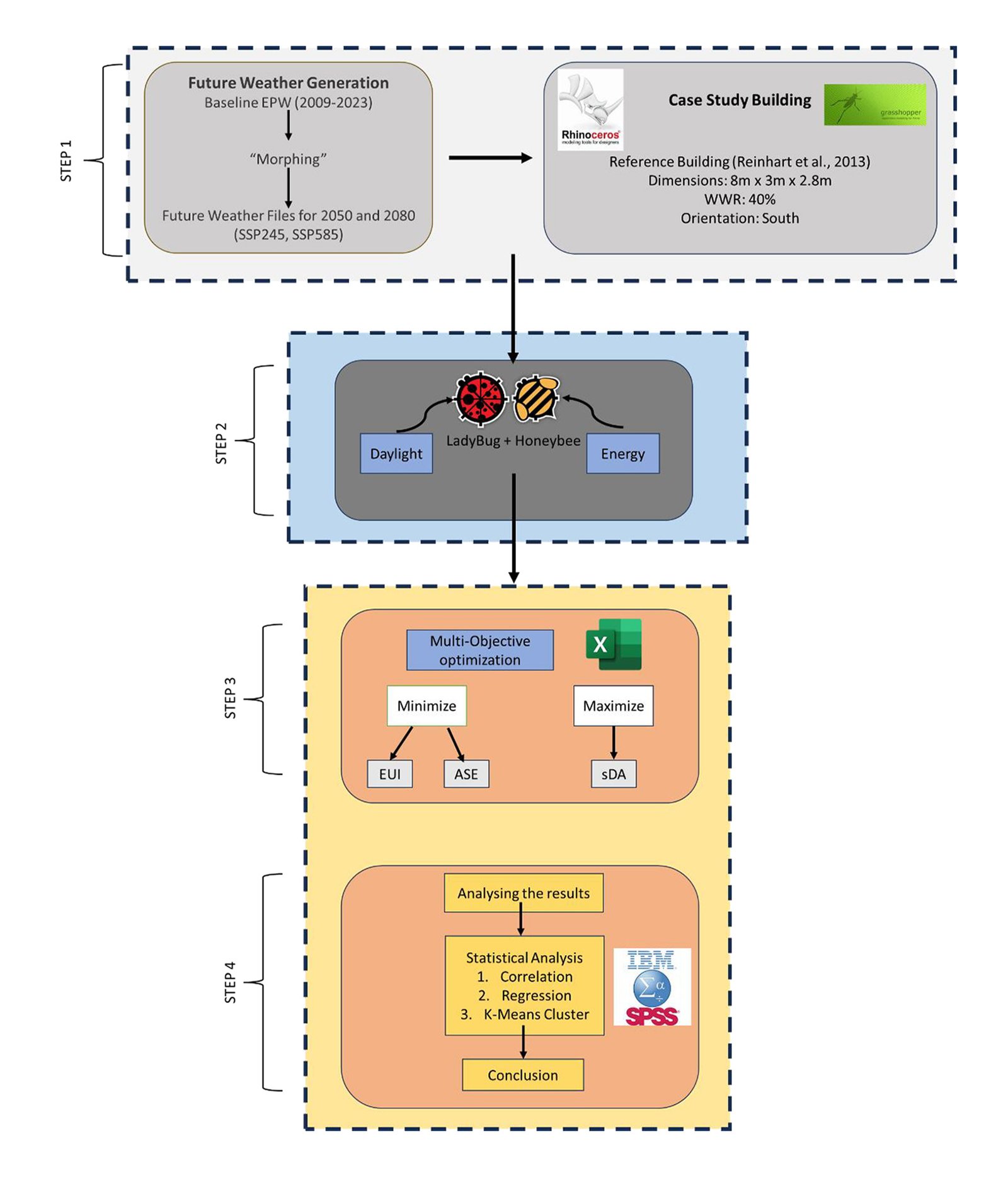
Fig. 1. Research Framework showing four sequential processes of climate data generation, parametric modeling, simulation, and optimization.
2.2. Future climate data generation
Future weather files for Kathmandu were generated using the Future Weather Generator [28], which implements the morphing methodology developed by Belcher et al. [33]. The baseline EnergyPlus Weather (EPW) file (2009-2023) was sourced from https://climate.onebuilding.org/. Two emission scenarios from CMIP6 were selected: SSP2-4.5 (Moderate emissions) and SSP5-8.5 (high emissions), for two time horizons: 2050 (near-future) and 2080 (far-future). The EC-Earth3 GCM was selected based on its high grid point density [28]. This yielded five weather files for simulation: present-day baseline, SSP2-4.5 2050, SSP2-4.5 2080, SSP5-8.5 2050, and SSP5-8.5 2080.
2.3. Case study building
The case study building is a reference room that is an office room which is based on Reinhart et al., [34] model (Fig. 2) and Table 1 summarizes the building simulation input parameters. The model has dimension of 3.9m x 8.5m x 2.8m (width x depth x height). This model has been by [35] and other researchers as well.
Figure 2
![Parametric Model of the Reference office room developed in Rhino Interface [34].](figures/13-315-2.jpg)
Fig. 2. Parametric Model of the Reference office room developed in Rhino Interface [34].
Table 1
Table 1. Building simulation parameters and inputs.
Only the southern façade was analyzed because southern side gets the most amount of sunlight each year. The model was made adiabatic that means no heat transfer occurs from other faces except for the south façade which has the window in it. The Window to Wall ratio was fixed at a value of 40%.
The rationale behind the selection of this value was office spaces need windows need to be big enough for sufficient daylight penetration and while Nepal doesn’t have its own fixed standard for WWR values, studies done in similar climate to Kathmandu like the ASHRAE Zone 4 (mixed climate) is generally at 40% or less and China’s GB 55015-2021 for Hot winter and Cold winter zone [36] which is analogous to Kathmandu’s temperate climate.
Generic in-built values for reflectance of the material were taken which were accessed from https://github.com/ladybug-tools/honeybee-standards/blob/master/honeybee_standards/modifiers/default.mat
2.4. Shading parameters
Horizontal shading devices were modelled as flat rectangular slats positioned above the window with two variable parameters. The louvers are equally spaced and the slats extend the full window width. Additionally, seven iterations of numbers of louvers (Count 0-6); 0 being no louvers and 6 being 6 equally spaced horizontal louvers were simulated to account for variations, resulting in a total of 210 simulations. Table 2 presents all the shading design parameters used for the study.
Table 2
Table 2. Shading design parameters used for parametric simulation.
2.5. Performance metrics
Three key performance metrics were calculated for each configuration:
- Energy Use Intensity: Total annual energy consumption for heating, cooling, and lighting per square meter (kWh/m2/yr). Lower values indicate better performance.
- Spatial Daylight Autonomy (sDA): The percentage of floor area receiving at least 300lux for at least 50% of the occupied hours. Higher values indicate better daylight coverage, with sDA ≥ 50% is generally considered a good indicative of good daylight performance.
- Annual Sunlight Exposure (ASE): The percentage of floor area receiving more than 1000lux of direct sunlight for at least 250 hours. Lower values indicate reduced glare risk, with ASE ≤ 10% generally considered acceptable.
2.6. Simulation tools and workflow
The simulation workflow integrates parametric modeling in Rhinoceros 3D/Grasshopper with validated simulation engines EnergyPlus and Radiance.
The base office room was modeled in Rhinoceros 3D version 7 using the Grasshopper parametric interface (Fig. 2 and Fig. 3). Shading depth, angle and the number of louvers were defined as variable parameters in Grasshopper using number sliders. EnergyPlus which is accessed via Ladybug Tools 1.8.0, was used to calculate EUI for each iteration. The weather file/ EnergyPlus weather (EPW) file for Kathmandu was downloaded from https://climate.onebuilding.org/. Radiance was accessed via Honeybee, was used for annual daylight simulations to calculate sDA and ASE. Table 3 summarizes the parameters that were used for daylighting simulation using radiance. The grid sensors were placed at a 0.5m spacing and at a height of 0.8m.
Figure 3
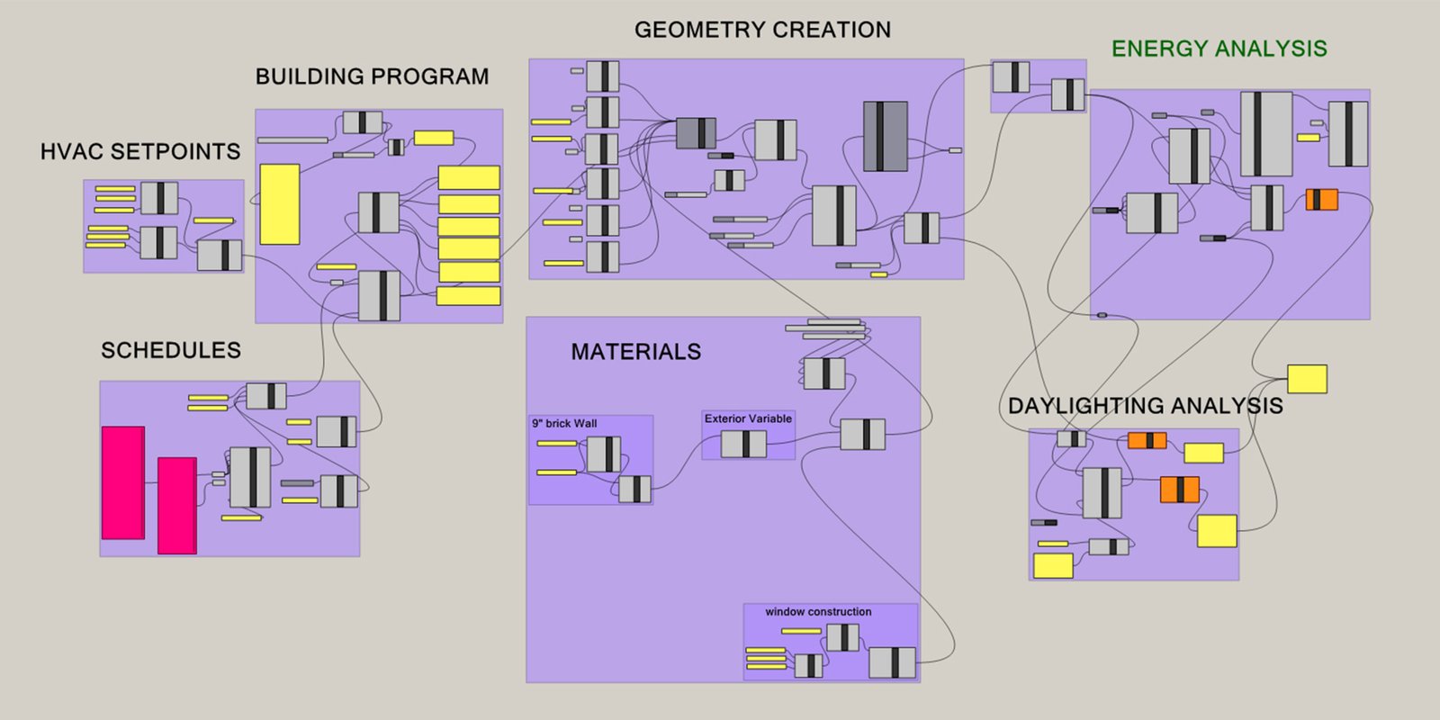
Fig. 3. Parametric Model of the Reference office room developed in Rhino Interface (Reinhart et al., 2013).
Table 3
Table 3. Shading design parameters used for parametric simulation.
2.7. Data compilation and multi object optimization
Pareto-optimal configurations were identified using pairwise dominance checking across three objectives: minimize EUI, maximize sDA, and minimize ASE. Configuration A dominates B if: 1) EUI_A ≤ EUI_B, 2) sDA_A ≥ sDA_B, 3) ASE_A ≤ ASE_B with at least one inequality strict.
The initial Pareto identification yielded 33 mathematically non-dominated configurations, each representing a unique combination of daylight and glare performance. This approach eliminates redundancy and ensures that the presented Pareto set reflects genuine performance trade-offs rather than duplicate design solutions.
2.7.1. Justification of pareto front identification method
The Pareto front was identified using Microsoft Excel rather than automated optimization algorithms (e.g., NSGA-II). This approach was appropriate because the study simulated all 210 possible configurations (7 counts × 5 depths × 6 angles), making complete enumeration possible. Because the discrete design space is fully enumerated, the exact Pareto front can be obtained by direct nondominated comparison rather than by an evolutionary algorithm such as NSGA-II, which is typically used to approximate Pareto-optimal sets [37,38]. The strong correlations observed between design parameters and performance metrics (Section 3.2.1) further confirm that the sampling density was sufficient to capture the underlying performance landscape. If the design space had been under sampled, such clear correlation patterns would not emerge. Additionally, the discrete nature of the variables (integer counts, 0.2m depth increments, 15° angle increments) means shading devices are built at specific dimensions, not continuous values, making exhaustive evaluation more appropriate than stochastic sampling. Excel-based pairwise dominance sorting also provides transparency and verifiability in how Pareto points were identified, which is advantageous when the design space is fully enumerated and well-understood.
2.8. Statistical analysis
Statistical analysis was carried out to validate the model and determine the relationships between various variables. The following statistical validation were carried out:
- Correlation Analysis: Pearson correlation coefficients were calculated using SPSS to understand relationships between design parameters (Count, Depth, Angle) and performance metrics (EUI, sDA, ASE).
- Multiple Regression Analysis: Two sets of regression analyses were conducted.
- First (Interdependence of metrics): Multiple linear regression was conducted with EUI as the dependent variable and sDA, ASE, Count, Depth, and Angle as independent variables. Variance inflation factors (VIF) were calculated to detect multicollinearity among predictors.
- Second (Sensitivity analysis): To identify which design parameters most influence each performance metric, three separate regression models were fitted with Count, Depth, and Angle as independent variables and EUI, sDA, and ASE as dependent variables, respectively. Standardized regression coefficients (β) were calculated to compare the relative influence of each design parameter across models.
- K-means Cluster analysis: To statistically validate groupings among Pareto-optimal configurations, K-means cluster analysis was performed using all six variables (EUI, sDA, ASE, Depth, Angle, Count). Variables were standardized to z-scores prior to analysis to ensure equal weighting. The optimal number of clusters (K=3) was determined through hierarchical cluster analysis using Ward's method. ANOVA was used to confirm significant differences between clusters.
3. Results and discussion
3.1. Climate data analysis
Under the moderate emissions scenario (SSP2-4.5), the annual mean temperature increases by 1.45°C by 2050 and 2.53°C by 2080. Under the high emissions scenario (SSP5-8.5), warming intensifies to 2.2°C by 2050 and 4.71°C by 2080. The warming shows significant seasonal variation, with winter months experiencing the largest absolute increases. Under SSP5-8.5 2080, January temperatures rise by 5.04°C (+50.9%), while June increases by 3.81°C (+16.0%). This differential warming has important implications for building energy performance, as winter demand decreases while cooling demand intensifies. Monthly DBT variation across different climatic scenarios is visualized in Fig. 4.
Figure 4
Fig. 4. Monthly Dry Bulb Temperature (DBT) for all climatic scenario (Baseline, SSP245 2050, SSP245 2080, SSP5852050, SSP5852080).
In addition to temperature, Global Horizontal Illuminance and Diffuse Horizontal Illuminance were also analyzed. Global Horizontal Illuminance decreases under future climate scenarios. Under SSP5-8.5 2080, annual illuminance shows a decrease of 10.9%. Monthly decreases range from 3.0% in January to 20.5% in August. Diffuse Horizontal Illuminance, however, shows an increase of 40.2% under the same scenario. Monthly diffuse increases range from 13.5% in August to 69.9% in February.
3.2. Overview of the simulation results
A total of 210 parametric simulations were successfully completed, covering all combinations of shading count (0-6), depth (0-0.8m), and angle (0-75°). The EUI ranges from 84.7-126.9 kWh/m²/yr, Spatial Daylight Autonomy sDA ranges 0 from 0-68.1%, and ASE ranges from 0-21.85. The wide range between maximum and minimum values demonstrate the significant impact of shading design has on both energy and daylight performance. These values illustrate the fundamental trade-off inherent in shading design: greater solar protection reduces energy consumption but also diminishes daylight availability and quality, while less shading improves daylight but also increases both energy use and glare risk. This trade-off has been extensively documented by [19,20,39].
3.2.1. Correlation analysis
Pearson correlation coefficients were calculated to understand relationships between design parameters and performance metrics (Table 4). We can see that the design parameters (Count, Depth, and Angle) show zero correlation with each other (r = 0.00), confirming that they are orthogonal design variables that can be designed independently. Depth is the most influential parameter, showing the strongest correlations with all three-performance metrics: EUI (r = -0.631; p < 0.01), ASE (r = -0.617; p < 0.01), and sDA (r = -0.570; p< 0.01). This aligns with findings by Kim et al. [14], who identified horizontal shading depth to reduce daylight and energy in south Korean buildings. Count (number of horizontal shading elements) is also of nearly equal influence with (EUI r = -0.605; p < 0.10), (ASE: r = -0.612; p , 0.01), and (sDA: r = -0.531; p < 0.01). whereas angle shows moderate correlation with sDA but weak, non-significant correlations with EUI and ASE, a finding consistent with Chou [40] and Lee et al. [41] that the angle of shading devices affects the amount of daylight entering the space, and when angled correctly can control glare and distribute light evenly across the room. The high correlations between sDA, ASE, EUI show that these parameters have strong interrelationships. Sherif et al. [13] reported similar correlations between sDA and ASE, validating these findings and reinforcing the necessity of multi objective optimization.
Table 4
Table 4. Shading design parameters used for parametric simulation.
** Correlation is significant at the 0.01 level (1-tailed)
* Correlation is significant at the 0.05 level (1-tailed)
3.2.2. Regression analysis
Model a: interdependence of performance metrics
Multiple linear regression was conducted to quantify the relative influence of design parameters and daylight metrics on energy performance. The regression model was highly significant (f(5, 204) = 1692.65, p < 0.001) and explained 97.6% of the variance in EUI (R2 = 0.976).
From Fig. 5 and Table 5 we can see that Daylight metrics dominate energy prediction: ASE (β = 0.616) and sDA (β = 0.366) are the strongest predictors of EUI, together accounting for the majority of explained variance. A one-unit increase in ASE corresponds to a 0.963 kWh/m2/yr increase in EUI, while one percentage point increase in sDA corresponds to a 0.254 kWh/m2/yr increase in EUI. This strong relationship confirms that energy consumption is primarily determined by daylight performance and buildings that admit more daylight inevitably consume more energy for cooling. This finding aligns with Viriezky et al. [42] that daylight can significantly increase the cooling loads without proper intervention. The variance inflation factors (VIF) reveal significant multicollinearity between the performance metrics: 1) ASE VIF = 5.176, 2) sDA VIF = 5.051.
Figure 5
Fig. 5. Standardized Beta Values Visualized for ASE, sDA, Depth, Count, Angle when EUI is taken as the dependent Variable.
Table 5

Table 5. Multiple linear regression analysis with EUI as dependent variable.
This indicates the ASE and sDA share substantial variance with each other and with EUI. This high interdependence means multi objective optimization is necessary. The strong interdependencies between the three-performance metrics mean that design decisions must balance all three objectives simultaneously. As Khoroshiltseva et al. [22] and Baghoolizadeh et al. [23] have demonstrated, Pareto-based multi-objective optimization is essential when dealing with such correlated performance metrics.
Model b: sensitivity analysis-influence of design parameters
To identify which design parameters most influence each performance metric, three separate regression models were fitted with Count, Depth, and Angle as independent variables. Table 6 presents the SRCs with EUI, sDA and ASE as separate dependent variables.
Depth consistently showed the strongest influence across all three models (β = -0.631 to -0.567, p < 0.01), followed by Count (β = -0.605 to -0.539, p < 0.01).
Table 6

Table 6. Sensitivity analysis- Design parameters as predictors.
Angle showed moderate influence only on sDA (β = -0.350, p < 0.01) and negligible influence on EUI (β = -0.142) and ASE (β = -0.066). This sensitivity analysis identifies shading depth and number of louvers as the most critical design parameters for balancing energy, daylight, and glare performance.
3.3. Multi objective optimization: Pareto front analysis
Given the strong interdependence between performance metrics, MOO is necessary. The Pareto front approach identifies non dominated solutions, where improving one objective would worsen at least one other objective. The three optimization objectives were: 1) Minimize EUI, 2) Maximize sDA, 3) Minimize ASE. All 210 data points are visualized in Fig. 6. The analysis identified 33 Pareto-optimal configurations out of 210 total simulations. Table 7 presents all Pareto optimal configurations, sorted on the basis of EUI (ascending).
Figure 6

Fig. 6. (a) 3D plot of all 210 points of EUI, sDA, and ASE. (b) 2D plot illustrating EUI and sDA.
Table 7

Table 7. All 33 Mathematically non-dominated solutions obtained from pair-wise dominance and filtering.
From Table 7 and Fig. 7 three distinct regions of performance can be visualized, each with characteristic trade-offs and design implications. To further validate the stratification, K-means clustering was performed.
Figure 7
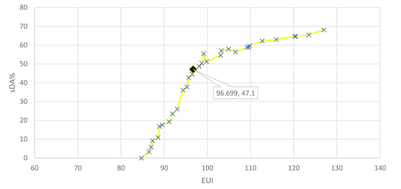
Fig. 7. Visual illustration of all 33 non-dominated and unconstrained optimal configurations.
3.4. Cluster analysis
Visual inspection of the Pareto form reveals a natural stratification of configurations based on their energy performance. When examining the 33 Pareto optimal configurations sorted by EUI, three distinct groups/regions appear as shown in Table 8.
To validate whether or not 3 distinct cluster of performance zones form—K-means cluster was used.
Table 8

Table 8. Visual Clustering of all 33 non-dominated solutions.
This machine learning technique partitions data into K-groups by minimizing within-cluster variance and maximizing between cluster differences. The analysis was conducted using all six variables: EUI, sDA (%), ASE, Depth (m), Angle (°), Count. All variables were standardized into z-scores prior to analysis to ensure equal weighting despite different units of measurement. The optimal number of clusters (K=3) was determined through hierarchical cluster analysis using Ward’s method, which clearly indicated a three-cluster solution as the most appropriate grouping.
Comparing Table 8 and Table 9 we can see that with every variable taken into account, the size of clusters somewhat changes with Figure 8 visualizing all 3 distinct clusters formed.
Figure 8
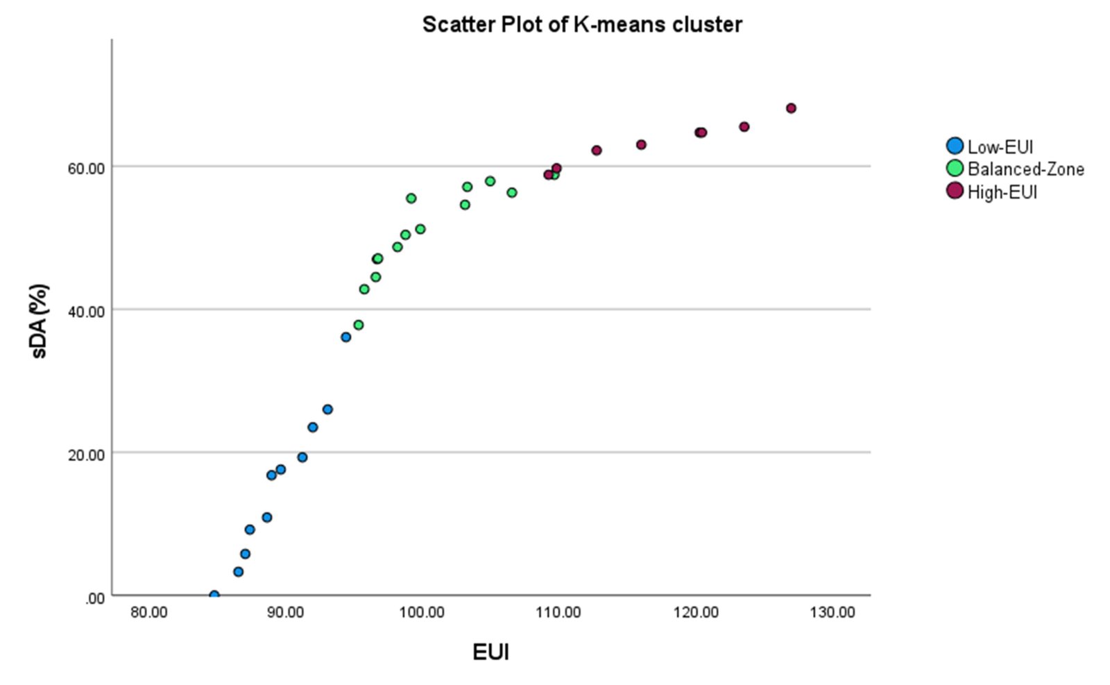
Fig. 8. Visual representation of K-means cluster of all 33 Unconstrained optimal configurations.
Table 9

Table 9. K-means Clustering of all 33 non-dominated solutions.
3.4.1. Region I: low EUI
From Table 9 IDs ranging from 1-11 fall within this zone. Configurations in this region employ deep shading (depth ≥ 0.6m) with steep angles and higher counts. EUI ranges from 84.7 to 94.352 kWh/m²/yr, representing energy savings of 27-33% compared to the unshaded baseline (129.6 kWh/m²/yr). sDA ranges from 0 to 36.1%, indicating minimal to low daylight coverage. The trade-off between maximum energy saving and daylight is clear. Remarkably, all the configurations in this region achieve ASE of 0. The deep shading prevents direct sunlight penetration, resulting in perfect glare protection.
This finding aligns with Atthaillah et al. [43], who demonstrated that shading depth beyond 2.0 m had diminishing returns on tropical daylit classrooms. Kim et al. [14] also concurs that longer the horizontal shade becomes, lower the intensity of indoor illuminance becomes.
3.4.2. Region II: balanced zone
Configurations ranging from ID 12-25 fall in this zone. This zone has the highest number of Pareto-optimal configurations (n=14).
This region features a diverse range of design parameters, with depths from 0.2m to 0.8m and angles from 0° to 30° with 0° horizontal configurations being more prominent, suggesting that horizontal louvers offer the best balance for south-facing façades. Counts range from 3 to 6 indicating that multiple shading elements are still beneficial. EUI ranges from 95.274 kWh/m²/yr to 109.184 kWh/m²/yr, representing energy savings of 14-25% compared to baseline. The progression shows a gradual increase in energy use as daylight improves. sDA ranges from 37.8% to 58.8%, encompassing the full spectrum from moderate to excellent daylight coverage. This region contains the configurations that achieve the best balance between energy and daylight. ASE values are generally low, ranging from 0 to 13.4, with many configurations maintaining zero glare. The first few configurations with non-zero ASE appear in this region. The “Knee point” (0.4m, 30°, Count 4) with EUI = 96.7 kWh/m2/yr, sDA = 47.1%, and ASE = 0.0 (Figure 9).
Figure 9
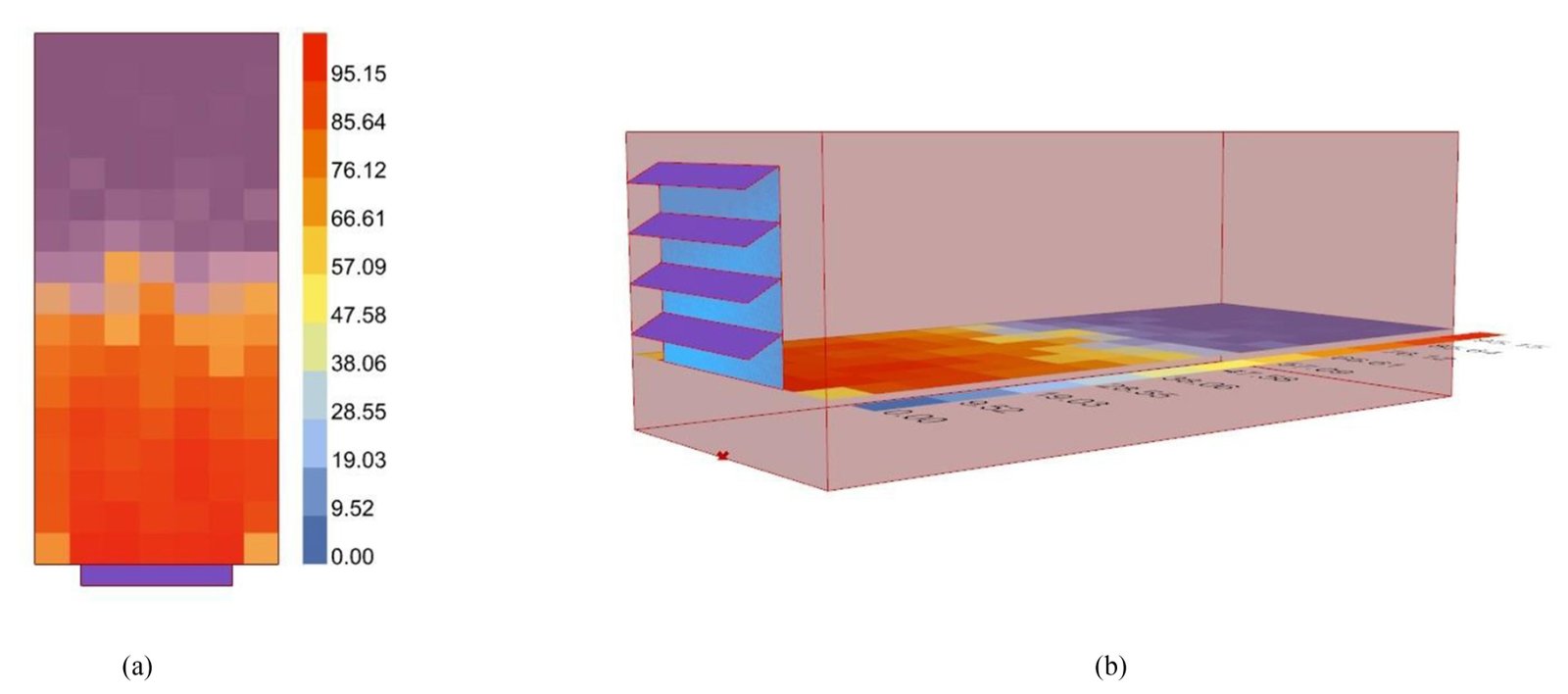
Fig. 9. (a) Top view of Daylight Autonomy. (b) Knee-Point (0.4m, 30°, Count 4) visual representation of shading devices.
The knee point is the point of maximum curvature where the tradeoff between energy and daylight changes most dramatically. To the left of this point, small increases in energy yield substantial improvements in daylight. Whereas, to the right of this point the gains in daylight diminish significantly. This is the theoretical point of best compromise between metrics [44].
Similar knee point identification and Pareto front analysis has been applied in building design optimization by Baghoolizadeh et al. [23], Zhang et al. [45], and Wu et al. [24], who noted that such points provide valuable guidance for efficient compromises. Configuration (0.4m, 0°, Count 6) with EUI = 99.8 kWh/m²/yr, sDA = 51.2%, and ASE = 0.0 represents the best overall balance among all Pareto-optimal configurations (Fig. 10). While the knee point is mathematically the most efficient, this configuration achieves notably higher daylight (51.2% vs. 47.1%) with only a modest energy penalty (+3.1 kWh/m²/yr, or about 3.2%) while maintaining perfect glare protection and achieving 21% energy reduction from baseline. This finding aligns with recommendations by Ramezani et al. [21], who found that horizontal shading devices with moderate depths provided optimal energy and daylight performance in hot-arid regions. Bahdad et al. [18] similarly demonstrated that optimized shading in Malaysian office buildings improved daylighting performance while maintaining reasonable energy consumption.
Figure 10
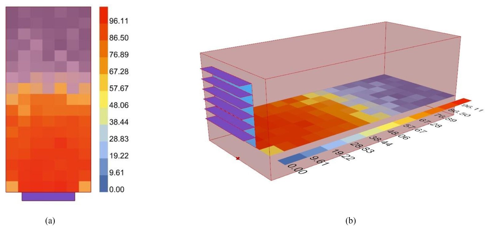
Fig. 10. (a) Top view of Daylight Autonomy. (b) Best Overall balance (0.4m, 0°, Count 6) visual representation of shading devices.
3.4.3. Region III: high EUI
A total of n=8 configurations fall in this zone (Table 9). The configurations in this region generally employs shading with low louver counts and shallower shading with most angles being horizontal (0°). Energy Use Intensity (EUI) ranging from 109.603 to 126.9 kWh/m²/yr, representing around 0-14% energy reduction from baseline. The unshaded configuration at the extreme right has no energy savings at all. sDA ranges from 58.8% to 68.1%, representing excellent daylighting. ASE values are high, ranging from 10.8 to 21.85. Region 3 configurations should only be considered when maximum daylight is absolutely required and glare can be managed through other means.
3.5. Constrained pareto front and zero-glare configurations
One finding of this study is that 18 of the 33 Pareto optimal configurations achieve zero glare (ASE = 0). While this is a somewhat interesting finding, most of these “zero-glare” configurations or mathematically non-dominated pareto front solutions lack practical feasibility, especially the configurations in the low-energy region as they are a byproduct of deep shading and provide inadequate daylighting to the studied space. This lack of practical feasibility aligns with Kovalerchuk [25] who noted that some solutions might lack real life applicability. Further filtering was done to get the Constrained Pareto Front (CPF) points. Applying a constraint of sDA ≥ 50% according to IES gave n = 16 (IDs 18-33) as the number of feasible pareto fronts which provide minimum required daylight illuminance shown in Table 10.
Table 10

Table 10. Table comparing Constrained and Unconstrained Pareto Front after applying constraint of sDA ≥ 50%.
The total number of non-dominated points decrease from 33 to 16 with all of the Region I and some of Region II being removed. The number of “zero-glare” points decrease from 18 to 3 when feasibility constraint is applied with all 3 “zero-glare” points in the Region II (Balanced-zone). This shows that zero glare designs that provide sufficient daylight are possible to achieve when optimized properly. This finding somewhat challenges the common assumption that good daylight and negligible glare are inherently conflicting and one cannot be achieved without compromising another. This statement that good daylight with sufficient glare protection can be achieved is also supported by several studies. Wienold et al. [46] who states that “healthy daytime lighting through daylight does not inherently increase glare risk and can be achieved without compromising visual comfort.” and De Luca et al. [47] in their study found that correctly designed exterior static shading can control sunlight and glare while providing adequate illuminance to the space. Similar findings also have been reported by Tabadkani et al. [3], who demonstrated that properly designed shading can simultaneously optimize multiple performance criteria.
3.6. Resilience testing of pareto front points under future climate scenarios
Five representative configurations (IDs 18, 20, 22, 25, 33) were taken from the 16 Constrained Pareto Optimal Points (sDA ≥ 50%). All five representative configurations were re-simulated under both scenarios for 2040 and 2080 time horizons. Table 11 presents the complete set of results.
Table 11

Table 11. Five representative configurations and EUI increase under different climatic scenarios.
Figure 11 represents the increase in EUI of selected representative points under different climatic scenarios [under SSP2-4.5 (2050), SSP2-4.5(2080), SSP5-8.5(2050), and SSP5-8.5(2080)]. Under SSP2-4.5, for overall balanced configuration i.e. ID 20, the increase is 17.5% and 28.3% for 2050 and 2080 from baseline and for SSP5-8.5 2050 and 2080, the increase is 22.8% and 45.6% respectively. Similarly for unshaded baseline (ID 33), the increase is 31.4% and 47.0% for SSP2-4.5 (2050 and 2080) and for SSP5-8.5 (2050 and 2080), the increase is 39.7% and 80.6% respectively. The increase is drastic under the worst-case scenario i.e. SSP 5-8.5 (2050 and 2080). The increase in EUI for both balanced point and unshaded baseline nearly double for SSP5-8.5 (2080) when compared to SSP2-4.5 (2080). This shows that increase in energy use of a space depends on projected climatic scenario. Multiple studies by Christenson et al. [48], Herrera et al. [49], Tarroja et al. [50] state that future climate projections can alter building energy demand, often increasing cooling loads and, in some climates, reducing heating loads, so the net effect depends on location, building type, and scenario. From Table 11 and Fig. 11 we can see that under worst-case warming (SSP5-8.5 2080), the unshaded baseline (ID 33) experiences an 80.6% increase in EUI, while optimized shading configurations experience substantially lower increases: ID 18 (+44.1%), ID 20 (+45.6%), and ID 22 (+47.8%). This demonstrates that optimized shading not only reduces present-day energy consumption but also significantly improves climate resilience, with well-designed shading configurations experiencing 30-35 percentage points lower energy increase than unshaded buildings.
Figure 11
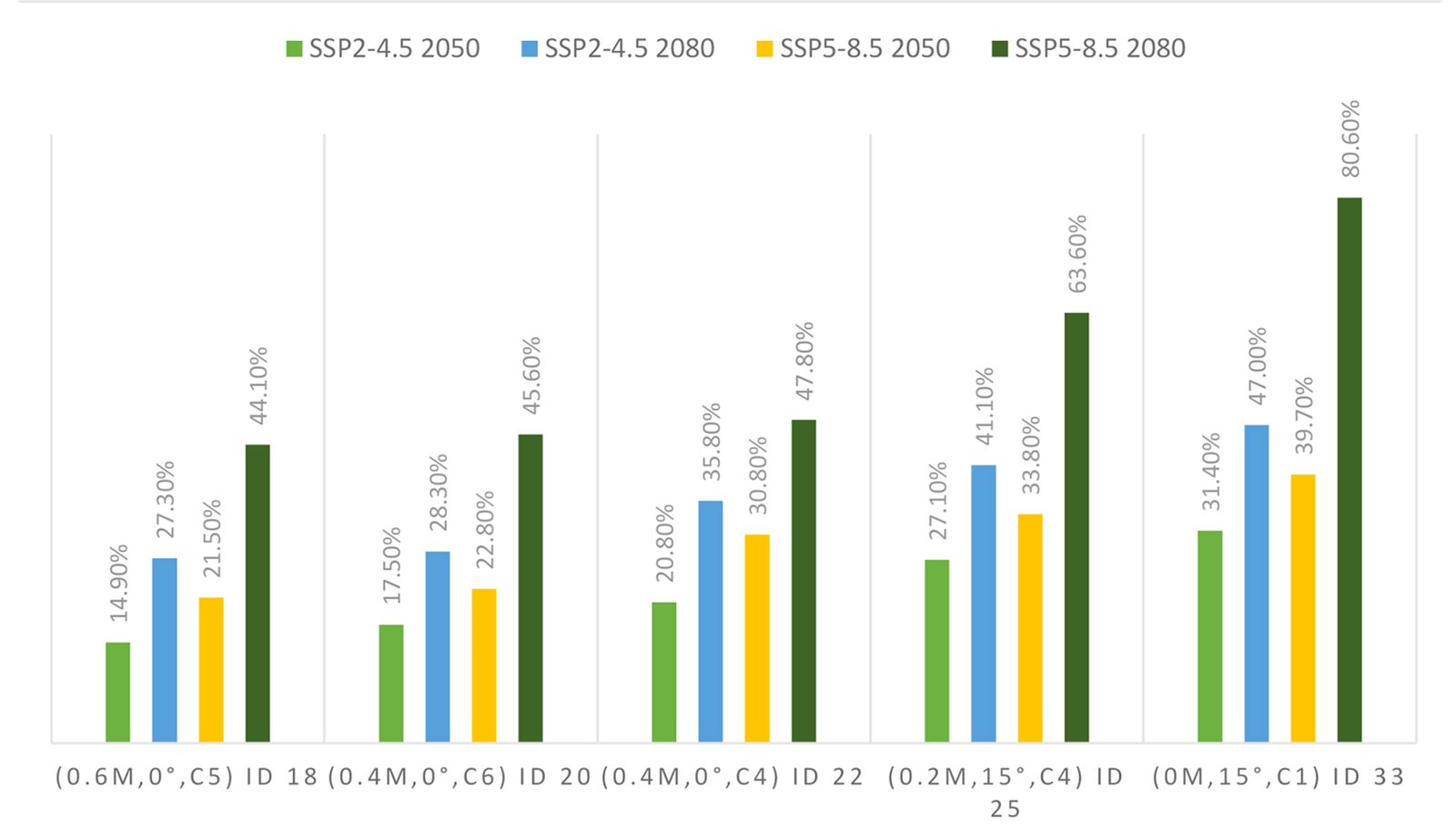
Fig. 11. Percentage Increase of EUI of 5 selected Pareto-Optimal Configurations across all four future climate scenarios (SSP245(2050), SSP245(2080), SSP585(2050), SSP585(2080)).
Another significant finding from this analysis is the consistent rightward shift of the entire Pareto front across all scenarios. Figure 12 presents the Pareto fronts for all four climatic scenarios (SSP2-4.5 2050, SSP2-4.5 2080, SSP5-8.5 2050, and SSP5-8.5 2080) and we can see a clear pattern, the shape of the front remains remarkably similar, but the entire curve shifts progressively to the right as the climate warming intensifies. This indicates that:
- The relative performance of configurations remains stable. Meaning that the configurations that perform well today continue to perform well in the future. This stability has clear implications: designers can optimize for present conditions with confidence that their choices will remain optimal under any future scenario.
- The same daylighting performance requires increasingly higher energy use as the climate warms. For example, achieving 50% sDA (ID 18) requires 98.71 kWh/m2/yr under present conditions, 113.374 kWh/m2/yr under SSP2-4.5 2050, and 142.199 kWh/m2/yr under SSP5-8.5 2080.
This progressive shift means that buildings designed to provide good daylight today will face substantially higher energy costs in the future.
- The widening range of EUI values across the Pareto front has important practical implications. The difference between the balanced and unshaded EUI (ID 33 - ID 20) expands from 27.169 kWh/m²/yr under present conditions to 84.046 kWh/m²/yr under SSP5-8.5 2080. This means that design choices become even more critical under future climate.
Figure 12
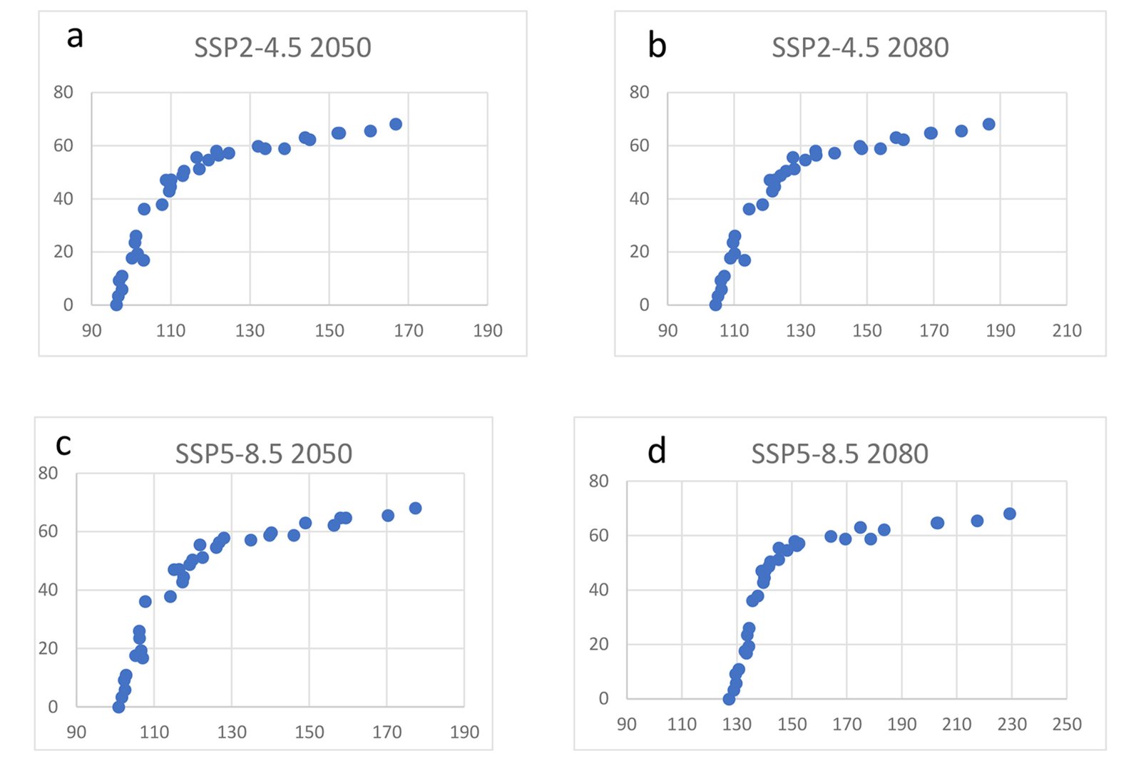
Fig. 12. Visual illustration of the rightward shift in Pareto Front Curve of All 33 Pareto Optimal Configurations. (a) SSP245 2050. (b) SSP245 2080. (c) SSP585 2050. (d) SSP585 2080.
The stability of the Pareto front shape can be attributed to two factors. First, sDA and ASE are geometry-based metrics calculated from annual sun positions and sky conditions. These metrics rely purely on the spatial configuration of facades, openings, and shading devices [51,52]. Therefore, each configuration maintains identical sDA and ASE values across all scenarios. Second, climate warming primarily increases cooling loads, which are proportional to a building’s exposure to solar gain [29].
These findings provide strong evidence that investments in quality and optimized shading provide compounding returns as the climate warms and that design decisions for shading design for present conditions will remain robust under future scenarios as well.
3.7. Design guidelines for south facing office facades in Kathmandu
Based on the comprehensive parametric analysis and multi-objective optimization (MOO), and future climate resilience analysis, the following set of recommendations have been recommended for south-facing office building façades. The five constrained configurations were taken and are presented in the Table 12 with the respective 3D visualization.
The key design principles that can be adopted are:
- Shading depth of 0.4m to 0.6m provide optimal balance for Kathmandu. Depths > 0.6m provides optimal balance whereas depths < 0.2m provide insufficient solar protection.
- Louver counts ranging from 4 to 6 are recommended. As count has nearly equal influence to depth on energy performance (β = -0.605).
- Tilt angle of 0° to 15° is recommended. Angle has minimal influence on energy and glare (β = -0.142 and -0.066), but moderate influence on daylight (β = -0.350).
- Distributing shading across multiple louvers is more effective than a single deep louver.
Table 12

Table 12. Summary of the Recommended Configurations and Performance.
3.8. Novelty and contribution
Several contributions are made. First multi-objective study for optimizing the horizontal shading devices in Kathmandu, providing evidence-based design guidelines for a rapidly urbanizing context. Second, it extends the literature for mathematically non-dominated solutions and practically feasible solutions. Third, this study also evaluates the resilience of design solutions under CMIP6 scenarios (SSP2-4.5 and SSP5-8.5) for 2050 and 2080, for Nepal, demonstrating that the energy advantage of optimized shading nearly triples under worst case warming and demonstrates that the design solution for present remain optimal through 2080.
4. Conclusion
This study conducted a comprehensive parametric simulation and multi-objective optimization of horizontal shading devices for south-facing office façades in Kathmandu, Nepal. A total of 210 simulations were performed, varying shading count (0-6), depth (0-0.8m), and angle (0-75°), with performance evaluated using Energy Use Intensity (EUI), Spatial Daylight Autonomy (sDA), and Annual Sunlight Exposure (ASE). The analysis identified 33 Pareto-optimal configurations; however, mathematical optimality does not guarantee practical suitability. When constrained by minimum daylight requirements (sDA ≥ 50%), the viable design space collapses to 16 feasible configurations, of which only 3 achieve zero glare (ASE = 0) : IDs 18, 20, and 21. K-means cluster analysis validated three distinct design strategies: Energy-Efficient (n=11) with deep shading achieving low EUI and zero glare but limited daylight; Balanced (n=14) with moderate shading achieving good daylight, low glare, and moderate EUI; and Daylight-Optimal (n=8) with minimal shading achieving high daylight but high EUI and significant glare risk. The recommended configuration is ID 20 (0.4 m depth, 0° angle, 6 louvers), achieving 51.2% sDA with zero glare and 21% energy savings. Under worst-case warming (SSP5-8.5 2080), ID 20 experiences a 46.5% EUI increase versus 80.6% for the unshaded baseline, demonstrating that optimized shading significantly improves climate resilience.
Under future climate scenarios, all configurations experience substantial EUI increases, but the magnitude varies significantly based on the configuration used. The best overall balance configuration increases from 99.8 to 145.2 kWh/m²/yr under worst-case 2080 which is a 45.5% increase that still leaves it 84.1 kWh/m²/yr lower than the unshaded alternative, an advantage that has nearly tripled from present conditions. The entire Pareto front shifts rightward while maintaining its shape, confirming that relative performance rankings remain stable and design decisions made today remain optimal under any future climate pathway. These findings provide evidence-based, climate-resilient design guidelines for Kathmandu's rapidly urbanizing context, demonstrating that investments in quality shading deliver compounding returns as the climate warms and that careful parametric optimization can identify configurations that successfully balance competing performance objectives both now and in the future.
4.1. Practical implementation of the design recommendations
4.1.1. Construction
- Specify the recommended balanced configuration (0.4m depth, 0° angle, 6 louvers, ID 20) as the default setting for south-facing office shading construction. This configuration achieves 51.2% sDA with zero glare and 21% energy savings.
- For daylight-critical projects (e.g. deep-floor plate offices, spaces with limited window area etc.) constrained configurations with higher sDA can be used with certain EUI and glare trade-off. Similarly, for projects where energy is the topmost priority, configurations with lower EUI can be used and for projects with visual comfort as priority, configurations with zero-glare can be used.
4.1.2. Building codes and policy
- Develop performance-based code provisions with quantifiable targets: sDA ≥ 50% (daylight autonomy), ASE ≤ 10% (glare protection), and EUI ≤ 100 kWh/m²/yr (energy performance) for south-facing office façades.
- Incentivize shading designs that simultaneously achieve all three targets: good daylight (sDA ≥ 50%), glare protection (ASE ≤ 10%), and energy savings (≥20% reduction compared to unshaded baseline).
- Require future climate considerations in energy modeling for buildings with expected lifespans beyond 2050, using at least SSP2-4.5 and SSP5-8.5 scenarios.
5. Limitations
This study has several limitations that should be considered when interpreting the findings. First, the analysis focused on south facing façades with a fixed window to wall ratio of 40 percent. Performance may differ for east and west orientations, which experience lower sun angles, and different window to wall ratios may alter the optimal shading configurations. Second, only static horizontal shading devices were simulated. Dynamic blinds or automated shading systems may achieve superior performance but may be too costly for Kathmandu's context. Fixed shading remains the most practical solution for widespread adoption in developing countries. Third, the future weather files were generated using a single General Circulation Model (EC Earth3), which does not capture the full range of climate model uncertainty. The use of multiple GCMs or ensemble approaches would provide a more robust assessment of future building performance. Fourth, this study used default Honeybee Radiance materials with fixed reflectance values: ceiling 0.80, walls 0.50, floor 0.20, and exterior shading device 0.35. The wall reflectance of 0.50 is lower than typical office standards, which may result in conservative or lower sDA predictions. Future research should conduct sensitivity analyses on surface reflectance values and, where possible, use measured local material properties. Fifth, the manual Pareto sorting method used in this study is not feasible for larger datasets with continuous variables. For such cases, algorithmic approaches such as NSGA-II would be more appropriate. The analysis also excluded view quality, life cycle cost, and embodied carbon of shading materials, which are factors essential for comprehensive design decision making. Finally, the study used a single reference office module. Results may differ for other building typologies with different occupancy patterns, internal loads, and floor plate depths. Future research should address these limitations through multi orientation analysis, dynamic system evaluation, life cycle assessment, and field validation studies.
Funding
This research received no external funding.
Author Contributions
The author confirms being the sole contributor of this work and has approved it for publication.
Declaration of competing interest
The authors declare no conflicts of interest.
References
- K. Kalaimathy, S. Gopalakrishnan, R. Shanthi Priya, C. Selvam, R. Senthil, Daylighting Strategies for Low-Rise Residential Buildings Through Analysis of Architectural Design Parameters, Architecture, 5:4 (2025) 125. https://doi.org/10.3390/architecture5040125
- N. Nasrollahi, E. Shokri, Daylight illuminance in urban environments for visual comfort and energy performance, Renewable and Sustainable Energy Reviews, 66 (2016) 861-874. https://doi.org/10.1016/j.rser.2016.08.052
- A. Tabadkani, A. Roetzel, H. X. Li, A. Tsangrassoulis, Daylight in Buildings and Visual Comfort Evaluation: the Advantages and Limitations, Journal of Daylighting, 8:2 (2021) 181-203. https://doi.org/10.15627/jd.2021.16
- C. Blume, C. Garbazza, M. Spitschan, Effects of light on human circadian rhythms, sleep and mood, Somnologie, 23:3 (2019) 147-156. https://doi.org/10.1007/s11818-019-00215-x
- L. Pérez-Lombard, J. Ortiz, C. Pout, A review on buildings energy consumption information, Energy and Buildings, 40:3 (2008) 394-398. https://doi.org/10.1016/j.enbuild.2007.03.007
- S. K. Alghoul, H. G. Rijabo, and M. E. Mashena, Energy consumption in buildings: A correlation for the influence of window to wall ratio and window orientation in Tripoli, Libya, Journal of Building Engineering, 11 (2017) 82-86. https://doi.org/10.1016/j.jobe.2017.04.003
- L. Pompei, L. Blaso, S. Fumagalli, F. Bisegna, The impact of key parameters on the energy requirements for artificial lighting in Italian buildings based on standard EN 15193-1:2017, Energy and Buildings, 263 (2022) 112025. https://doi.org/10.1016/j.enbuild.2022.112025
- Z. Afroz, M. Goldsworthy, S. D. White, Energy flexibility of commercial buildings for demand response applications in Australia, Energy and Buildings, 300 (2023) 113533. https://doi.org/10.1016/j.enbuild.2023.113533
- R. Singh, I. J. Lazarus, V. V. N. Kishore, Uncertainty and sensitivity analyses of energy and visual performances of office building with external venetian blind shading in hot-dry climate, Applied Energy, 184 (2016) 155-170. https://doi.org/10.1016/j.apenergy.2016.10.007
- A. Nezamdoost, K. Van Den Wymelenberg, A daylighting field study using human feedback and simulations to test and improve recently adopted annual daylight performance metrics, Journal of Building Performance Simulation, 10:5-6 (2017) 471-483. https://doi.org/10.1080/19401493.2017.1334090
- L. Heschong, K. Van Den Wymelenberg, M. Andersen, N. Digert, L. Fernandes, A. C. Keller, J. Loveland, H. McKay, R. G. Mistrick, B. Mosher, C. Reinhart, Z. Rogers, M. Tanteri, Approved method: IES Spatial Daylight Autonomy (sDA) and Annual Sunlight Exposure (ASE), Infoscience, Ecole Polytechnique Fédérale De Lausanne, 2012. [Online]. Available: http://infoscience.epfl.ch/record/196436
- M. Ayoub, A multivariate regression to predict daylighting and energy consumption of residential buildings within hybrid settlements in hot-desert climates, Indoor and Built Environment, 28:6 (2019) 848-866. https://doi.org/10.1177/1420326X18798164
- N. Sherif, A. Yehia, W. S. E. Ismaeel, Simulation and Statistical Validation Method for Evaluating Daylighting Performance in Hot Climates, Urban Science, 9:8 (2025) 303. https://doi.org/10.3390/urbansci9080303
- S.-H. Kim, K.-J. Shin, H.-J. Kim, Y.-H. Cho, A Study on the Effectiveness of the Horizontal Shading Device Installation for Passive Control of Buildings in South Korea, International Journal of Polymer Science, 2017 (2017) 1-11. https://doi.org/10.1155/2017/3025092
- Md. J. Rana, Md. R. Hasan, Md. H. R. Sobuz, An investigation on the impact of shading devices on energy consumption of commercial buildings in the contexts of subtropical climate, SASBE, 11:3 (2022) 661-691. https://doi.org/10.1108/SASBE-09-2020-0131
- F. De Luca, H. Voll, M. Thalfeldt, Horizontal or vertical? Windows' layout selection for shading devices optimization, MEQ, 27:6 (2016) 623-633. https://doi.org/10.1108/MEQ-05-2015-0102
- F. F. Hernández, J. M. Cejudo López, J. M. Peña Suárez, M. C. González Muriano, S. C. Rueda, Effects of louvers shading devices on visual comfort and energy demand of an office building. A case of study, Energy Procedia, 140 (2017) 207-216. https://doi.org/10.1016/j.egypro.2017.11.136
- A. A. S. Bahdad, S. F. S. Fadzil, N. Taib, Optimization of Daylight Performance Based on Controllable Light-shelf Parameters using Genetic Algorithms in the Tropical Climate of Malaysia, Journal of Daylighting, 7:1 (2020) 122-136. https://doi.org/10.15627/jd.2020.10
- S. G. Koç, S. Maçka Kalfa, The effects of shading devices on office building energy performance in Mediterranean climate regions, Journal of Building Engineering, 44 (2021) 102653. https://doi.org/10.1016/j.jobe.2021.102653
- P. Esquivias, C. Munoz, I. Acosta, D. Moreno, J. Navarro, Climate-based daylight analysis of fixed shading devices in an open-plan office, Lighting Research & Technology, 48:2 (2016) 205-220. https://doi.org/10.1177/1477153514563638
- M. Ramezani, S. Taheri, M. S. Gorgabi, A. Nourbakhsh Sadabad, Energy and daylighting trade-offs in residential window design: multi-objective optimization for hot-arid regions, Sci Rep, 16:1 (2025) 3458. https://doi.org/10.1038/s41598-025-33473-x
- M. Khoroshiltseva, D. Slanzi, I. Poli, A Pareto-based multi-objective optimization algorithm to design energy-efficient shading devices, Applied Energy, 184 (2016) 1400-1410. https://doi.org/10.1016/j.apenergy.2016.05.015
- M. Baghoolizadeh, M. Rostamzadeh-Renani, R. Rostamzadeh-Renani, D. Toghraie, Multi-objective optimization of Venetian blinds in office buildings to reduce electricity consumption and improve visual and thermal comfort by NSGA-II, Energy and Buildings, 278 (2023) 112639. https://doi.org/10.1016/j.enbuild.2022.112639
- Z. Wu, Y. Xu, Z. Wang, Multi-objective optimization of energy, view, daylight and thermal comfort for building's fenestration and shading system in hot-humid climates, PLoS One, 20:6 (2025) e0325290. https://doi.org/10.1371/journal.pone.0325290
- B. Kovalerchuk, Pareto Front and General Line Coordinates, in: Visual Knowledge Discovery and Machine Learning, vol. 144, Springer International Publishing: Cham, Switzerland, 2018, pp. 277-287. https://doi.org/10.1007/978-3-319-73040-0_11
- V. Eyring, S. Bony, G. A. Meehl, C. A. Senior, B. Stevens, R. J. Stouffer, K. E. Taylor, Overview of the Coupled Model Intercomparison Project Phase 6 (CMIP6) experimental design and organization, Geosci. Model Dev., 9:5 (2016) 1937-1958. https://doi.org/10.5194/gmd-9-1937-2016
- G. Evola, L. Marletta, D. Cimino, Weather data morphing to improve building energy modeling in an urban context, MMEP, 5:3 (2018) 211-216. https://doi.org/10.18280/mmep.050312
- E. Rodrigues, M. S. Fernandes, D. Carvalho, Future weather generator for building performance research: An open-source morphing tool and an application, Building and Environment, 233 (2023) 110104. https://doi.org/10.1016/j.buildenv.2023.110104
- J. Mu, Y. Feng, D. Yang, G. Yang, CMIP6 climate change and wind environment impacts on cold-region residential energy and thermal comfort: A case study of Harbin, Energy for Sustainable Development, 90 (2026) 101885. https://doi.org/10.1016/j.esd.2025.101885
- G. S. M. Viganò, R. Rugani, M. Marengo, M. Picco, Assessing the Impact of Climate Change on Building Energy Performance: A Future-Oriented Analysis on the UK, Architecture, 4:4 (2024) 1201-1224. https://doi.org/10.3390/architecture4040062
- National Statistics Office, National Population and Housing Census 2021 Provincial Report (BAGMATI PROVINCE), National Statistics Office, 2021.
- B. Basnet, S. Uprety, A Pilot Study on the Effect of Daylighting and Orientation in the Office Building: A Case of Kathmandu, Adv. Engin. & Technol., 2:01 (2022) 33-45. https://doi.org/10.3126/aet.v2i01.50435
- S. Belcher, J. Hacker, D. Powell, Constructing design weather data for future climates, Building Services Engineering Research and Technology, 26:1 (2005) 49-61. https://doi.org/10.1191/0143624405bt112oa
- C. Reinhart, A. Jakubiec, D. Ibarra, Definition Of A Reference Office For Standardized Evaluations Of Dynamic Facade And Lighting Technologies, in: Proceedings of the 2017 Building Simulation Conference, 26 August 2013. https://doi.org/10.26868/25222708.2013.1029
- M. Mahdavinejad, S. M. H. Ayatollahi, S. Motevali, P. Norouzi, A. Kari, B. Ghasemi, The impact of facade geometry on visual comfort and energy consumption in an office building in different climates, Energy Reports, 11 (2024) 1-17. https://doi.org/10.1016/j.egyr.2023.11.021
- X. Meng, Y. Meng, J. Nunoshige, Theoretical energy-saving potential assessment of an office building renovated to comply with GB 55015-2021 across three China climate zones, in: Proceedings of the 2025 Building Simulation Conference, August 2025. https://doi.org/10.26868/25222708.2025.1403
- Xiao-Bing Hu, Ming Wang, E. Di Paolo, Calculating Complete and Exact Pareto Front for Multiobjective Optimization: A New Deterministic Approach for Discrete Problems, IEEE Trans. Cybern., 43:3 (2013) 1088-1101. https://doi.org/10.1109/TSMCB.2012.2223756
- K. Deb, A. Pratap, S. Agarwal, T. Meyarivan, A fast and elitist multiobjective genetic algorithm: NSGA-II, IEEE Trans. Evol. Computat., 6:2 (2002) 182-197. https://doi.org/10.1109/4235.996017
- N. Kunwar, M. Bhandari, A comprehensive analysis of energy and daylighting impact of window shading systems and control strategies on commercial buildings in the United States, Energies, 13:9 (2020) 2401. https://doi.org/10.3390/en13092401
- Chia-Peng Chou, The Performance of Daylighting with Shading Device in Architecture Design, 淡江理工學刊, 7:4 (2004). https://doi.org/10.6180/jase.2004.7.4.02
- K. Lee, K. Han, J. Lee, The Impact of Shading Type and Azimuth Orientation on the Daylighting in a Classroom-Focusing on Effectiveness of Façade Shading, Comparing the Results of DA and UDI, Energies, 10:5 (2017) 635. https://doi.org/10.3390/en10050635
- V. Viriezky, O. C. Dewi, A. M. Dugar, Lighting Energy Reduction by Optimizing Daylight while Maintaining Cooling Load in Tropical Educational Building, Depok, Indonesia, J. Sustain. Archit. Civ. Eng., 32:1 (2023) 145-161. https://doi.org/10.5755/j01.sace.32.1.32267
- Atthaillah, R. A. Mangkuto, M. D. Koerniawan, B. Yuliarto, On the Interaction between the Depth and Elevation of External Shading Devices in Tropical Daylit Classrooms with Symmetrical Bilateral Openings, Buildings, 12:6 (2022) 818. https://doi.org/10.3390/buildings12060818
- W. Li, G. Zhang, T. Zhang, S. Huang, Knee Point-Guided Multiobjective Optimization Algorithm for Microgrid Dynamic Energy Management, Complexity, 2020 (2020) 1-11. https://doi.org/10.1155/2020/8877008
- J. Zhang, L. Zhang, P. Ren, W. Hao, A. Xu, Multi-objective optimization prediction model for building parameters of photovoltaic windows based on NSGA II-BP, Case Studies in Thermal Engineering, 64 (2024) 105500. https://doi.org/10.1016/j.csite.2024.105500
- J. Wienold, M. Sabeti, V. R. M. Lo Verso, DO CIE-RECOMMENDATIONS FOR PROPER LIGHT AT THE PROPER TIME CONFLICT WITH GLARE?, in: CIE x051:2025 Proceedings of the CIE 2025 Midterm Meeting, Vienna, Austria, 7-9 July 2025, pp. 1208-1216. https://doi.org/10.25039/x051.2025/x5gzpg
- F. De Luca, A. Sepúlveda, T. Varjas, Multi-performance optimization of static shading devices for glare, daylight, view and energy consideration, Building and Environment, 217 (2022) 109110. https://doi.org/10.1016/j.buildenv.2022.109110
- M. Christenson, H. Manz, D. Gyalistras, Climate warming impact on degree-days and building energy demand in Switzerland, Energy Conversion and Management, 47:6 (2006) 671-686. https://doi.org/10.1016/j.enconman.2005.06.009
- M. Herrera, S. Natarajan, D. A. Coley, T. Kershaw, A. P. Ramallo-González, M. Eames, D. Fosas, M. Wood, A review of current and future weather data for building simulation, Building Services Engineering Research and Technology, 38:5 (2017) 602-627. https://doi.org/10.1177/0143624417705937
- B. Tarroja, F. Chiang, A. Aghamohammadi, S. Zhang, B. D. Solomon, S. Samuelsen, Translating climate change and heating system electrification impacts on building energy use to future greenhouse gas emissions and electric grid capacity requirements in California, Applied Energy, 225 (2018) 522-534. https://doi.org/10.1016/j.apenergy.2018.05.003
- A. Ruiz, M. Á. Campano, I. Acosta, Ó. Luque, Partial Daylight Autonomy (DAp): A New Lighting Dynamic Metric to Optimize the Design of Windows for Seasonal Use Spaces, Applied Sciences, 11:17 (2021) 8228. https://doi.org/10.3390/app11178228
- C. Bauer, S. Wittkopf, Annual Daylight Simluations With EvalDRC: Assessing The Performance Of Daylight Redirecting Components, Journal of Facade Design and Engineering, (2016) 253-272. https://doi.org/10.3233/FDE-160044
2383-8701/© 2026 The Author(s). Published by solarlits.com. This is an open access article distributed under the terms and conditions of the Creative Commons Attribution 4.0 License.

618
Total views
Citations
SHARE ON


